Fitting hierarchical distance sampling models in spAbundance
Jeffrey W. Doser, Marc Kéry
2023 (last update: March 21, 2024)
Source:vignettes/distanceSampling.Rmd
distanceSampling.RmdIntroduction
This vignette provides worked examples and explanations for fitting
single-species and multi-species hierarchical distance sampling (HDS)
models in the spAbundance R package. We will provide step
by step examples on how to fit the following models:
- HDS model using
DS(). - Spatial HDS model using
spDS(). - Multi-species HDS model using
msDS(). - Multi-species HDS model with species correlations using
lfMsDS(). - Spatial multi-species HDS model with species correlations using
sfMsDS().
In this vignette we are only describing spAbundance
functionality to fit HDS models, with separate vignettes on fitting
N-mixture models and generalized linear mixed models. We fit all models
in a Bayesian framework using custom Markov chain Monte Carlo (MCMC)
samplers written in C/C++ and called through
R’s foreign language interface. Here we will provide a
brief description of each model, with full statistical details provided
in a separate vignette. As with all model types in
spAbundance, we will show how to perform posterior
predictive checks as a Goodness of Fit assessment, model comparison and
assessment using the Widely Applicable Information Criterion (WAIC), and
out-of-sample predictions using standard R helper functions (e.g.,
predict()). Note that syntax of distance sampling models in
spAbundance closely resembles syntax for fitting occupancy
models in spOccupancy (Doser et al.
2022), and that this vignette closely follows the documentation
on the spOccupancy
website.
To get started, we load the spAbundance package, as well
as the coda package, which we will use for some MCMC
summary and diagnostics. We will also use functions in the
stars, ggplot2, and unmarked
packages to create some basic plots of our results. We then set a seed
so you can reproduce the same results as we do.
Example data set: Birds in the southeastern US
As an example data set throughout this vignette, we will use distance
sampling data from the National Ecological Observatory Network (NEON).
Here we use data on 16 bird species collected in 2018 in the Disney
Wilderness Preserve in Florida, USA. Briefly, data were collected at 90
sites where observers recorded the number of all bird species observed
during a six-minute, unlimited radius point count survey once during the
breeding season. Distance of each individual bird to the observer was
recorded using a laser rangefinder. For modeling, we binned the distance
measurements into 4 intervals (0-25, 25-50, 50-100, 100-250), removing
all observations >250m away. We removed all species with less than 10
observations, leaving us with 16 species observed across the 90 sites.
More on the study location can be found on the NEON
website. The data are provided as part of the
spAbundance package and are loaded with
data(neonDWP). See the manual page using
help(neonDWP) for more information on the species included
in the data. Note that the neonDWP data set was updated in
spAbundance v0.1.1 after NEON discovered an error in the
processing of the data (more details here),
and so if you are running this vignette with spAbundance
v0.1.0 you will get slightly different results.
List of 5
 $ y          : num [1:16, 1:90, 1:4] 0 0 0 0 0 0 1 0 0 0 ...
  ..- attr(*, "dimnames")=List of 3
  .. ..$ : chr [1:16] "EATO" "EAME" "AMCR" "BACS" ...
  .. ..$ : NULL
  .. ..$ : NULL
 $ covs       :'data.frame':    90 obs. of  4 variables:
  ..$ wind  : int [1:90] 0 0 0 1 0 0 1 0 0 1 ...
  ..$ day   : num [1:90] 132 132 132 132 132 132 132 132 132 129 ...
  ..$ forest: num [1:90] 0.18 0.0962 0.0577 0.1569 0.08 ...
  ..$ grass : num [1:90] 0.2 0.192 0.192 0.216 0.22 ...
 $ dist.breaks: num [1:5] 0 0.025 0.05 0.1 0.25
 $ offset     : num 19.6
 $ coords     : num [1:90, 1:2] 458629 458879 459129 458629 458879 ...
  ..- attr(*, "dimnames")=List of 2
  .. ..$ : NULL
  .. ..$ : chr [1:2] "easting" "northing"
The object neonDWP is a list that is structured in the
format needed for multi-species distance sampling in
spAbundance. Specifically, neonDWP is a list
comprised of the distance sampling data for the 16 species
(y), covariates to include on either abundance and/or
detection (covs), the break points of the distance bands
(dist.breaks), an offset (offset), and the
spatial coordinates for each site (coords). Note the
coordinates are only required for spatially-explicit HDS models. The
three-dimensional array y consists of the distance sampling
data for all 16 species in the data set, where the dimensions of
y correspond to species (16), sites (90), and distance band
(4). For single-species distance sampling models in Section 2 and 3, we
will only use data for the Eastern Towhee (EATO), so we next subset the
neonDWP list to only include data from EATO in a new object
dat.EATO.
sp.names <- dimnames(neonDWP$y)[[1]]
dat.EATO <- neonDWP
dat.EATO$y <- dat.EATO$y[sp.names == "EATO", , ]
# Number of EATO individuals observed at each site
apply(dat.EATO$y, 1, sum)
[1] 2 1 2 3 1 0 0 2 3 2 1 2 2 3 2 2 2 3 2 1 1 1 2 2 0 3 1 3 3 0 1 4 0 0 0 1 2 0
[39] 0 1 0 0 1 0 0 0 2 2 1 3 2 3 4 3 1 1 3 2 0 2 1 1 2 4 3 2 4 3 3 7 5 5 1 0 2 0
[77] 3 2 2 1 1 2 1 0 0 0 0 2 0 1We see that EATO appears to be quite common across the 90 sites.
Single-species HDS models
Let \(N_j\) be the true abundance of the species of interest at site \(j = 1, \dots, J\). Following the HDS model introduced by Royle, Dawson, and Bates (2004), we model abundance following
\[\begin{equation} N_j \sim \text{Poisson}(\mu_jA_j), \end{equation}\]
where \(\mu_j\) is the expected
abundance at site \(j\) and \(A_j\) is an offset. In distance sampling,
the offset term will usually correspond to some measure of area sampled,
hence the use of the notation \(A_j\).
Note that with this definition, if an area offset is supplied when
fitting the model, the estimates of \(\mu_j\) will correspond to abundance per
unit area (i.e., density), while the estimates of \(N_j\) correspond to point-level abundance,
regardless of whether or not an offset is supplied. Note that
spAbundance also supports a negative binomial distribution
for abundance, which will have an additional dispersion parameter \(\kappa\), such that low values of \(\kappa\) denote large amounts of
overdispersion, and as \(\kappa \rightarrow
\infty\), the NB model becomes the Poisson distribution.
We model \(\mu_j\) as a function of spatially-varying covariates with a log link function. More specifically, we have
\[\begin{equation} \text{log}(\mu_j) = \boldsymbol{x}_j^\top\boldsymbol{\beta}, \end{equation}\]
where \(\boldsymbol{\beta}\) is a vector of effects for covariates in \(\boldsymbol{x}_j\) (including an intercept)
We assume data come from observers that count the number of individuals of the species at any given location (i.e., a line transect or point count survey) and record the distance to the line/center of the point count survey of each bird within a set of \(k = 1, \dots, K\) distance bands. Note that if continuous distances are reported, they can be post-hoc binned into a set of \(K\) distance bands and fit with the package. Define \(\boldsymbol{y}_j\) as a vector of \(K\) values indicating the number of individuals observed within each distance band \(k\) at site \(j\). Similarly, let \(\boldsymbol{y}^\ast_j\) be a vector of \(K + 1\) values, where the first \(K\) values correspond to \(\boldsymbol{y}_j\), and the last value is the number of unobserved individuals at that location (i.e., \(N_j - \sum_{k = 1}^Ky_{k, j}\).) Note that the last value in \(\boldsymbol{y}^\ast_j\) is not observed (i.e., since \(N_j\) is not known). We model \(\boldsymbol{y}^\ast_j\) according to
\[\begin{equation} \boldsymbol{y}^\ast_j \sim \text{Multinomial}(N_j, \boldsymbol{\pi}_j^\ast), \end{equation}\]
where \(\boldsymbol{\pi}_j^\ast\) is a vector of \(K + 1\) cell-specific detection probabilities with the first \(K\) values denoted as \(\boldsymbol{\pi}_j\) and the last value \(\pi^\ast_{j, K + 1} = 1 - \sum_{k = 1}^K\pi_{j, k}\). More specifically, the \(k\)th value in \(\boldsymbol{\pi}_j\), \(\pi_{j, k}\), is the probability of detecting an individual in the \(k\)th distance band at site \(j\). We define \(\pi_{j, k}\) as
\[\begin{equation} \pi_{j, k} = \bar{p}_{j, k}\psi_{k}, \end{equation}\]
where \(\bar{p}_{j, k}\) is the probability of detecting an individual in distance band \(k\) at site \(j\), given the individual occurs in distance band \(k\), and \(\psi_{k}\) is the probability an individual occurs in distance band \(k\). Following the standard distance sampling assumption that animals are uniformly distributed in space, for line transects, we have
\[\begin{equation} \psi_{k} = \frac{b_{k + 1} - b_k}{B}, \end{equation}\]
where \(b_{k + 1}\) and \(b_k\) are the upper and lower distance limits for band \(k\), and \(B\) is the line transect half-width. Additionally for line transects, we have
\[\begin{equation} \bar{p}_{j, k} = \frac{1}{B}\int_{b_k}^{b_{k+1}}g(\text{x})d\text{x}. \end{equation}\]
For circular point count transects, we have
\[\begin{equation} \psi_k = \frac{b^2_{k + 1} - b^2_k}{B^2}, \end{equation}\]
where \(b_{k + 1}\) and \(b_k\) are similarly the upper and lower distance limits for band \(k\), and \(B\) is the radius of the full point count circle. We then define \(\bar{p}_{j, k}\) as
\[\begin{equation} \bar{p}_{j, k} = \frac{1}{B^2}\int_{b_k}^{b_{k+1}}g(\text{x})2\text{x}d\text{x}. \end{equation}\]
For both line transects and point count surveys, \(g(\text{x})\) is some function of distance
\(\text{x}\) from the transect
line/center of point count survey. spAbundance currently
supports two detection functions: half-normal and negative exponential.
Both of these functions are governed by a scale parameter \(\sigma_j\), which can vary across sites to
allow detection probability to vary across spatial locations. We can
then model \(\sigma_j\) as
\[\begin{equation} \text{log}(\sigma_j) = \boldsymbol{v}_j^\top\boldsymbol{\alpha}, \end{equation}\]
where \(\boldsymbol{\alpha}\) is a vector of regression coefficients for covariates \(\boldsymbol{v_j}\) (including an intercept).
To complete the Bayesian specification of the model, we assign normal priors to the abundance (\(\boldsymbol{\beta}\)) and detection (\(\boldsymbol{\alpha}\)) regression coefficients, and a uniform prior for the negative binomial overdispersion parameters (if applicable).
Fitting single-species HDS models with DS()
The DS() function fits single-species distance sampling
models. DS() has the following arguments:
DS(abund.formula, det.formula, data, inits, priors, tuning,
   n.batch, batch.length, accept.rate = 0.43, family = 'Poisson',
   transect = 'line', det.func = 'halfnormal',
   n.omp.threads = 1, verbose = TRUE,
   n.report = 100, n.burn = round(.10 * n.batch * batch.length), n.thin = 1,
   n.chains = 1, ...)
The first two arguments, abund.formula and
det.formula, use standard R model syntax to denote the
covariates to be included in the abundance and detection portions of the
model, respectively. Only the right hand side of the formulas are
included. Random intercepts and slopes can be included in both the
abundance and detection portions of the HDS model using
lme4 syntax (Bates et al.
2015). For example, to include a random intercept for different
observers in the detection portion of the model, we would include
(1 | observer) in the det.formula, where
observer indicates the specific observer for each data
point. See the N-mixture modeling vignette for an example of fitting
models in spAbundance with random effects. The names of
variables given in the formulas should correspond to those found in
data, which is a list consisting of the following tags:
y (distance sampling data), covs (covariates),
dist.breaks (breakpoints for distance bands),
offset (an optional offset), and coords.
y should be stored as a sites x distance bin matrix,
covs is a matrix or data frame with site-specific covariate
values, dist.breaks is a vector of length equal to the
number of columns in y plus one comprised of distances that
denote the breakpoints of the distance bands, and offset is
an offset that can be used to scale estimates from abundance per survey
to density per some desired unit of measure. The dat.EATO
list is already in the required format. Note that we have four
covariates in covs, which includes an ordinal measure of
the amount of wind during the survey (0 is low, 3 is high), the day the
survey took place, and the amount of forest cover and grassland cover
within a 1km radius circle around the point count location. Here we will
model abundance as a function of forest and grassland cover, and model
detection probability as a linear function of wind (and of course by
distance, since that is what distance sampling does). Note that although
wind is measured as an ordinal variable, here we make the
simplifying assumption that the effect of wind on detection probability
takes a linear relationship as the ordinal variable increases, which
reduces the number of parameters we need to estimate. Notice that we use
the scale() function to standardize all the coefficients in
the model such that their mean is 0 and standard deviation is 1. This is
often useful for obtaining convergence of our MCMC models.
Notice the dist.breaks element in dat.EATO
consists of five values:
dat.EATO$dist.breaks[1] 0.000 0.025 0.050 0.100 0.250These values correspond to the distance cut off values (in km) for
the 4 distance bins in our distance sampling data. An important point to
mention is that when fitting distance sampling models in
spAbundance, the models can be somewhat sensitive to
initial values of the detection parameters, which is a result of the
initial values resulting in an invalid likelihood. This is particularly
true when the distance breaks take large values (e.g., 100). Thus, we
recommend converting the units of distance breaks to a value that is as
small as possible, but still makes sense. For example, we originally
calculated the distance breaks values for this data set in meters, but
we then divided them by 1000 to give the distance break values in km
instead. Note that if bad initial values are supplied to a distance
sampling model, the underlying functions will select new initial values
that do not result in an invalid likelihood, and so this will generally
not be a problem that you encounter when fitting a model, but there
could be situations when the functions do not successfully catch bad
initial values.
The offset in this case takes value 19.63, which will
put the estimated regression coefficients on the scale of individuals
per ha rather than individuals per point count. To see where the value
comes from, recall we are using 250m (.25km) radius point count surveys
and that the area of a circle is \(\pi
r^2\), with \(r\) being the
circle’s radius. To get our estimates on a per hectare scale, we set our
offset to the area in km\(^2\) then
multiply it by 100.
# Offset to switch from km2 to ha
radius.km <- .25
pi * radius.km^2 * 100[1] 19.63495Next, we specify the initial values for the MCMC sampler in
inits. DS() (and all other
spAbundance model fitting functions) will set initial
values by default, but here we will do this explicitly, since in more
complicated cases setting initial values close to the presumed solutions
can be vital for success of an MCMC-based analysis. The default initial
values for abundance regression coefficients (including the intercepts)
are random values from a standard normal distribution. The initial
values for the detection regression coefficients are random values from
a Uniform(-10, 10) distribution. If an invalid starting value for the
detection regression coefficients is drawn (or specified by the user),
spAbundance will report a message saying it is trying a
different starting value (also drawn randomly from a Uniform(-10, 10)),
and will continue to do so until it finds values that do not result in
an invalid likelihood. The default initial values for the latent
abundance effects are set to the total number of individuals observed at
that site. When fitting a HDS model with a negative binomial
distribution, the initial value for the overdispersion parameter is
drawn from the prior distribution. Initial values are specified in a
list with the following tags: N (latent abundance values),
alpha (detection intercept and regression coefficients),
beta (abundance intercept and regression coefficients), and
kappa (negative binomial overdispersion parameter). Below
we set all initial values of the regression coefficients to 0, initial
values for the overdispersion parameter to 1, and set initial values for
N to the total number of observed individuals at each site.
For the abundance (beta) and detection (alpha)
regression coefficients, the initial values are passed either as a
vector of length equal to the number of estimated parameters (including
an intercept, and in the order specified in the model formula), or as a
single value if setting the same initial value for all parameters
(including the intercept). Below we take the latter approach. For the
negative binomial overdispersion parameter, the initial value is simply
a single numeric value. To specify the initial values for the latent
abundance at each site (N), we must ensure we set the value
to at least the total number of individuals observed at a site, because
we know the true abundance must be greater than or equal to the number
of individuals observed (i.e., assuming no false positives). If the
initial values for N do not meet this criterion,
DS() will fail. spAbundance will provide a
clear error message if the supplied initial values for N
are invalid. Below we use the raw count data and the
apply() function to set the initial values.
We next specify the priors for the abundance and detection regression
coefficients, as well as the negative binomial overdispersion parameter.
We assume normal priors for both the detection and abundance regression
coefficients. These priors are specified in a list with tags
beta.normal for abundance and alpha.normal for
detection parameters (including intercepts). Each list element is then
itself a list, with the first element of the list consisting of the
hypermeans for each coefficient and the second element of the list
consisting of the hypervariances for each coefficient. Alternatively,
the hypermean and hypervariances can be specified as a single value if
the same prior is used for all regression coefficients. By default,
spAbundance will set the hypermeans to 0 and the
hypervariances to 100. For the negative binomial overdispersion
parameter, we will use a uniform prior. This prior is specified as a tag
in the prior list called kappa.unif, which should be a
vector with two values indicating the lower and upper bound of the
uniform distribution. The default prior is to set the lower bound to 0
and the upper bound to 100. Recall that lower values of
kappa indicate substantial overdispersion and high values
of kappa indicate minimal overdispersion. If there is
little support for overdispersion when fitting a negative binomial
model, we will likely see the estimates of kappa be close
to the upper bound of the uniform prior distribution. For the default
prior distribution, if the estimates of kappa are very
close to 100, this indicates little support for overdispersion in the
model, and we can likely switch to using a Poisson distribution (which
would also likely be favored by model comparison approaches). Below we
use default priors for all parameters, but specify them explicitly for
clarity.
prior.list <- list(beta.normal = list(mean = 0, var = 100),
alpha.normal = list(mean = 0, var = 100),
kappa.unif = c(0, 100))The next four arguments (tuning, n.batch,
batch.length, and accept.rate) are all related
to the specific type of MCMC sampler we use when we fit HDS models in
spAbundance. The parameters in HDS models are all estimated
using whats called a Metropolis-Hastings step, which can often be slow
and inefficient, leading to slow mixing and convergence of the MCMC
chains. To try and mitigate the slow mixing and convergence issues, we
update all parameters using an algorithm called an adaptive
Metropolis-Hastings algorithm (see Roberts and
Rosenthal (2009) for more details on this algorithm). In this
approach, we break up the total number of MCMC samples into a set of
“batches”, where each batch has a specific number of MCMC samples. Thus,
we must specify the total number of batches (n.batch) as
well as the number of MCMC samples each batch contains
(batch.length) when specifying the function arguments. The
total number of MCMC samples is n.batch * batch.length.
Typically, we set batch.length = 25 and then play around
with n.batch until convergence of all model parameters is
reached. We generally recommend setting batch.length = 25,
but in certain situations this can be increased to a larger number of
samples (e.g., 100), which can result in moderate decreases in run time.
Here we set n.batch = 2000 for a total of 50,000 MCMC
samples for each MCMC chain we run.
n.batch <- 2000
batch.length <- 25
# Total number of MCMC samples per chain
batch.length * n.batch[1] 50000Importantly, we also need to specify a target acceptance rate and
initial tuning parameters for the abundance and detection regression
coefficients (and the negative binomial overdispersion parameter and any
latent random effects if applicable). These are both features of the
adaptive algorithm we use to sample these parameters. In this adaptive
Metropolis-Hastings algorithm, we propose new values for the parameters
from some proposal distribution, compare them to our previous values,
and use a statistical algorithm to determine if we should accept the new
proposed value or keep the old one. The accept.rate
argument specifies the ideal proportion of times we will accept the
newly proposed values for these parameters. Roberts and Rosenthal (2009) show that if we
accept new values around 43% of the time, this will lead to optimal
mixing and convergence of the MCMC chains. Following these
recommendations, we should strive for an algorithm that accepts new
values about 43% of the time. Thus, we recommend setting
accept.rate = 0.43 unless you have a specific reason not to
(this is the default value). The values specified in the
tuning argument help control the initial values we will
propose for the abundance/detection coefficients and the negative
binomial overdispersion parameter. These values are supplied as input in
the form of a list with tags beta, alpha, and
kappa. The initial tuning value can be any value greater
than 0, but we generally recommend starting the value out around 0.5.
These tuning values can also be thought of as tuning “variances”, as it
is these values that controls the variance of the distribution we use to
generate newly proposed values for the parameters we are trying to
estimate. In short, the new values that we propose for the parameters
beta, alpha, and kappa come from
a normal distribution with mean equal to the current value for the given
parameter and the variance equal to the tuning parameter. Thus, the
smaller this tuning parameter/variance is, the closer our proposed
values will be to the current value, and vise versa for large values of
the tuning parameter. The “ideal” value of the tuning variance will
depend on the data set, the parameter, and how much uncertainty there is
in the estimate of the parameter. This initial tuning value that we
supply is the first tuning variance that will be used for the given
parameter, and our adaptive algorithm will adjust this tuning parameter
after each batch to yield acceptance rates of newly proposed values that
are close to our target acceptance rate that we specified in the
accept.rate argument. Information on the acceptance rates
for a few of the parameters in our model will be displayed when setting
verbose = TRUE. After some initial runs of the model, if
you notice the final acceptance rate is much larger or smaller than the
target acceptance rate (accept.rate), you can then change
the initial tuning value to get closer to the target rate. While use of
this algorithm requires us to specify more arguments than if we didn’t
“adaptively tune” our proposal variances, this leads to much shorter run
times compared to a more simple approach where we do not have an
“adaptive” sampling approach, and it should thus save us time in the
long haul when waiting for these models to run. For our example here, we
set the initial tuning values to 0.5 for beta,
alpha, and kappa.
tuning <- list(beta = 0.5, alpha = 0.5, kappa = 0.5)
# accept.rate = 0.43 by default, so we do not specify it.We also need to specify the length of burn-in (n.burn),
the rate at which we want to thin the posterior samples
(n.thin), and the number of MCMC chains to run
(n.chains). Note that currently spAbundance
runs multiple chains sequentially and does not allow chains to be run
simultaneously in parallel across multiple threads. Instead, we allow
for within-chain parallelization using the n.omp.threads
argument. We can set n.omp.threads to a number greater than
1 and smaller than the number of threads on the computer you are using.
Generally, setting n.omp.threads > 1 will not result in
decreased run times for non-spatial models in spAbundance,
but can substantially decrease run time when fitting spatial models
(Finley, Datta, and Banerjee 2020). Here
we set n.omp.threads = 1, and run the model for three
chains to assess convergence using the Gelman-Rubin diagnostic (Rhat;
Brooks and Gelman (1998)).
n.burn <- 20000
n.thin <- 30
n.chains <- 3The family argument is used to indicate whether we want
to model abundance with a Poisson distribution (Poisson) or
a negative binomial distribution (NB). Here we will start
with a Poisson distribution (the default), which we will compare to a
model with a negative binomial distribution later. The
det.func argument is used to specify the specific detection
function to use for allowing detection probability to vary by distance.
spAbundance currently supports two functions: half-normal
(halfnormal) and negative exponential
(negexp). Here we will use a half-normal detection
function, but we could of course compare this function to a negative
exponential using model selection criteria. The transect
argument is used to specify whether the distance sampling data come from
linear transects (line) or circular transects
(point). Finally, the verbose argument is a
logical value indicating whether or not MCMC sampler progress is
reported to the screen. If verbose = TRUE, sampler progress
is reported to the screen. The argument n.report specifies
the interval to report the Metropolis-Hastings sampler acceptance rate.
Note that n.report is specified in terms of batches, not
the overall number of samples. Below we set n.report = 500,
which will result in information on the acceptance rate and tuning
parameters every 500th batch (not sample).
We now are set to fit the model.
out <- DS(abund.formula = abund.formula,
det.formula = det.formula,
data = dat.EATO,
n.batch = n.batch,
batch.length = batch.length,
inits = inits.list,
family = 'Poisson',
det.func = 'halfnormal',
transect = 'point',
tuning = tuning,
priors = prior.list,
accept.rate = 0.43,
n.omp.threads = 1,
verbose = TRUE,
n.report = 500,
n.burn = n.burn,
n.thin = n.thin,
n.chains = n.chains)----------------------------------------
Preparing to run the model
----------------------------------------
----------------------------------------
Model description
----------------------------------------
Poisson HDS model with 90 sites.
Samples per Chain: 50000 (2000 batches of length 25)
Burn-in: 20000
Thinning Rate: 30
Number of Chains: 3
Total Posterior Samples: 3000
Source compiled with OpenMP support and model fit using 1 thread(s).
Adaptive Metropolis with target acceptance rate: 43.0
----------------------------------------
Chain 1
----------------------------------------
Sampling ...
Batch: 500 of 2000, 25.00%
Parameter Acceptance Tuning
beta[1] 48.0 0.05376
beta[2] 60.0 0.05270
beta[3] 44.0 0.05709
alpha[1] 44.0 0.07706
alpha[2] 36.0 0.07862
-------------------------------------------------
Batch: 1000 of 2000, 50.00%
Parameter Acceptance Tuning
beta[1] 56.0 0.05485
beta[2] 72.0 0.05063
beta[3] 36.0 0.05376
alpha[1] 40.0 0.07257
alpha[2] 56.0 0.08348
-------------------------------------------------
Batch: 1500 of 2000, 75.00%
Parameter Acceptance Tuning
beta[1] 44.0 0.05709
beta[2] 44.0 0.05596
beta[3] 32.0 0.05485
alpha[1] 40.0 0.08021
alpha[2] 36.0 0.08689
-------------------------------------------------
Batch: 2000 of 2000, 100.00%
----------------------------------------
Chain 2
----------------------------------------
Sampling ...
Batch: 500 of 2000, 25.00%
Parameter Acceptance Tuning
beta[1] 32.0 0.05596
beta[2] 44.0 0.05376
beta[3] 28.0 0.05063
alpha[1] 52.0 0.08021
alpha[2] 44.0 0.08348
-------------------------------------------------
Batch: 1000 of 2000, 50.00%
Parameter Acceptance Tuning
beta[1] 52.0 0.05270
beta[2] 68.0 0.05485
beta[3] 32.0 0.05376
alpha[1] 40.0 0.07706
alpha[2] 56.0 0.08689
-------------------------------------------------
Batch: 1500 of 2000, 75.00%
Parameter Acceptance Tuning
beta[1] 48.0 0.05709
beta[2] 56.0 0.05596
beta[3] 48.0 0.05376
alpha[1] 68.0 0.06835
alpha[2] 40.0 0.08348
-------------------------------------------------
Batch: 2000 of 2000, 100.00%
----------------------------------------
Chain 3
----------------------------------------
Sampling ...
Batch: 500 of 2000, 25.00%
Parameter Acceptance Tuning
beta[1] 56.0 0.04963
beta[2] 20.0 0.05063
beta[3] 36.0 0.04865
alpha[1] 32.0 0.08348
alpha[2] 20.0 0.09043
-------------------------------------------------
Batch: 1000 of 2000, 50.00%
Parameter Acceptance Tuning
beta[1] 40.0 0.05485
beta[2] 60.0 0.05166
beta[3] 48.0 0.05709
alpha[1] 40.0 0.07554
alpha[2] 28.0 0.08183
-------------------------------------------------
Batch: 1500 of 2000, 75.00%
Parameter Acceptance Tuning
beta[1] 44.0 0.05596
beta[2] 48.0 0.05063
beta[3] 24.0 0.05376
alpha[1] 32.0 0.08183
alpha[2] 56.0 0.08689
-------------------------------------------------
Batch: 2000 of 2000, 100.00%DS() returns a list of class DS with a
suite of different objects, many of them being coda::mcmc
objects of posterior samples. The “Preparing to run the model” section
will print information on default priors or initial values that are used
when they are not specified in the function call. Here we specified
everything explicitly so no information was reported.
We next use the summary() function on the resulting
DS() object for a concise, informative summary of the
regression parameters and convergence of the MCMC chains.
summary(out)
Call:
DS(abund.formula = abund.formula, det.formula = det.formula,
data = dat.EATO, inits = inits.list, priors = prior.list,
tuning = tuning, n.batch = n.batch, batch.length = batch.length,
accept.rate = 0.43, family = "Poisson", transect = "point",
det.func = "halfnormal", n.omp.threads = 1, verbose = TRUE,
n.report = 500, n.burn = n.burn, n.thin = n.thin, n.chains = n.chains)
Samples per Chain: 50000
Burn-in: 20000
Thinning Rate: 30
Number of Chains: 3
Total Posterior Samples: 3000
Run Time (min): 0.2785
Abundance (log scale):
Mean SD 2.5% 50% 97.5% Rhat ESS
(Intercept) 0.2146 0.1225 -0.0325 0.2169 0.4602 1.0113 211
scale(forest) 0.2337 0.0845 0.0690 0.2349 0.3980 1.0302 451
scale(grass) -0.0067 0.0823 -0.1669 -0.0069 0.1548 1.0102 496
Detection (log scale):
Mean SD 2.5% 50% 97.5% Rhat ESS
(Intercept) -3.0971 0.0438 -3.1823 -3.0973 -3.0128 1.0094 422
scale(wind) -0.0912 0.0334 -0.1553 -0.0917 -0.0261 1.0006 3000Notice both the abundance and detection coefficients are printed on the log scale. Recall that since we included an offset in the data list, the abundance values are on the scale of individuals per ha. Thus, at average values of forest cover and grassland, our model estimates there are exp(0.21) individuals per ha, which is 1.24. We also see a positive effect of forest cover on EATO density, and essentially no effect of grassland.
The model summary also provides information on convergence of the
MCMC chains in the form of the Gelman-Rubin diagnostic (Brooks and Gelman 1998) and the effective
sample size (ESS) of the posterior samples. Here we find all Rhat values
are less than 1.1 and the ESS values are substantially large for all
parameters. The ESS values are also adequately high for all model
parameters, indicating adequate mixing of the MCMC chains. We can
further look at traceplots of different parameters to get a better sense
of convergence. This can be done using the plot() function,
which has three arguments for all spAbundance models:
x (the resulting object from fitting the model),
param (the parameter name that you want to display), and
density (a logical value indicating whether to also
generate a density plot in addition to the traceplot). To see the
parameter names available to use with plot() for a given
model type, you can look at the manual page for the function, which for
models generated from DS() can be accessed with
?plot.DS.
Below we generate a traceplot for the three abundance coefficients.
plot(out, param = 'beta', density = FALSE)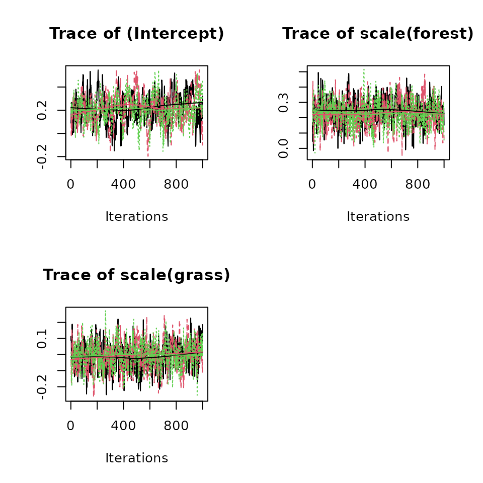
Looking at the detection portion of the model summary, we see there
is a negative effect of wind on detection probability, indicating that
as wind increases, detection probability decreases, which is what we
would expect. Interpreting the intercept detection parameter is a bit
difficult and doesn’t itself provide us with a great understanding of
how detection varies with distance. Instead, we can plot the
relationship between distance and detection using our estimated
parameter value. The below code generates a plot of detection
probability versus distance (at the average value of wind). Notice we
use the nifty gxhn() function from unmarked to
get the estimated detection probability value for a given distance and
scale parameter value when using the half normal function (see
?gxhn for more details).
det.int.samples <- out$alpha.samples[, 1]
det.quants <- quantile(exp(out$alpha.samples[, 1]), c(0.025, 0.5, 0.975))
x.vals <- seq(0, .125, length.out = 200)
n.vals <- length(x.vals)
p.plot.df <- data.frame(med = gxhn(x.vals, det.quants[2]),
low = gxhn(x.vals, det.quants[1]),
high = gxhn(x.vals, det.quants[3]),
x.val = x.vals * 1000)
ggplot(data = p.plot.df) +
geom_ribbon(aes(x = x.val, ymin = low, ymax = high), fill = 'grey',
alpha = 0.5) +
theme_bw(base_size = 14) +
geom_line(aes(x = x.val, y = med), col = 'black', linewidth = 1.3) +
labs(x = 'Distance (m)', y = 'Detection Probability')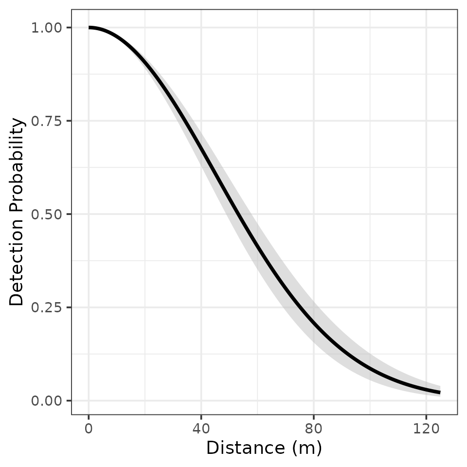
We see detection probability of EATO is quite high up to fairly moderate distances away from the observer (detection probability is 0.5 at about 55m away). This is perhaps not too surprising given the very distinctive “drink-your-tea” song of EATO.
Posterior predictive checks
The function ppcAbund() performs a posterior predictive
check on all spAbundance model objects as a Goodness of Fit
(GoF) assessment. The fundamental idea of GoF testing is that a good
model should generate data that closely align with the observed data. If
there are drastic differences in the true data from the model generated
data, our model is likely not very useful (Hobbs
and Hooten 2015). In spAbundance, we perform
posterior predictive checks using the following approach:
- Fit the model using any of the model-fitting functions (here
DS()), which generates replicated values for all observed data points. - Optionally bin both the actual and the replicated count data in some manner, such as by site.
- Compute a fit statistic on both the actual data and also on the model-generated ‘replicate data’.
- Compare the fit statistics for the true data and replicate data. If they are widely different, this suggests a lack of fit of the model to the actual data set at hand.
We calculate the replicate values in two steps. We first predict a value of latent abudance at each site using the expected abundance at site \(j\) for each MCMC sample \(l\) (i.e., \(\mu^{(l)}_j\)), and then subsequently generate the estimated counts in each distance bin \(k\) at that site \(j\). More specifically, the replicate values are calculated as
\[\begin{equation} \begin{split} N^{(l)}_{\text{rep}, j} &\sim \text{Poisson}(\mu^{(l)}_j), \\ \boldsymbol{y}^{(l)}_{\text{rep}, j} &\sim \text{Multinomial}(N^{(l)}_{\text{rep}, j}, \boldsymbol{\pi}^{(l)}_j). \end{split} \end{equation}\]
Note the Poisson distribution is replaced with a negative binomial distribution if that is used to fit the model. This is what we call a “marginal” approach to calculating replicate data values. See our discussion in the N-mixture modeling vignette for further details on different approaches to calculating replicate values in hierarchical models.
To perform a posterior predictive check, we send the resulting
DS model object as input to the ppcAbund()
function, along with a fit statistic (fit.stat) and a
numeric value indicating how to group, or bin, the data
(group). Currently supported fit statistics include the
Freeman-Tukey statistic and the Chi-Squared statistic
(freeman-tukey or chi-squared, respectively,
Kéry and Royle (2016)). For HDS models,
ppcAbund() allows the user to group the data by row (site;
group = 1) or not at all (group = 0).
ppcAbund() will then return a set of posterior samples for
the fit statistic (or discrepancy measure) using the actual data
(fit.y) and model generated replicate data set
(fit.y.rep), summed across all data points in the chosen
manner. For example, when setting group = 1,
spAbundance will first sum all of the count values at a
given site across all distance bands at that site, then calculate the
fit statistic using the site-level sums. When setting
group = 0, spAbundance calculates the fit
statistic directly on the count value in each site and distance bin.
The resulting values from a call to ppcAbund() can be
used with the summary() function to generate a Bayesian
p-value, which is the probability, under the fitted model, to obtain a
value of the fit statistic that is more extreme (i.e., larger) than the
one observed, i.e., for the actual data. Bayesian p-values are sensitive
to individual values, so we may also want to explore the discrepancy
measures for each (potentially “grouped”) data point.
ppcAbund() returns a matrix of posterior quantiles for the
fit statistic for both the observed (fit.y.group.quants)
and model generated, replicate data
(fit.y.rep.group.quants) for each “grouped” data point.
We next perform a posterior predictive check using the Freeman-Tukey
statistic grouping the data by sites. We summarize the posterior
predictive check with the summary() function, which reports
a Bayesian p-value. A Bayesian p-value that hovers around 0.5 indicates
adequate model fit, while values less than 0.1 or greater than 0.9
suggest our model does not fit the data well (Hobbs and Hooten 2015). As always with a
simulation-based analysis using MCMC, you will get numerically slightly
different values.
Call:
ppcAbund(object = out, fit.stat = "freeman-tukey", group = 1)
Samples per Chain: 50000
Burn-in: 20000
Thinning Rate: 30
Number of Chains: 3
Total Posterior Samples: 3000
Bayesian p-value: 0.474
Fit statistic: freeman-tukey The Bayesian p-value is greater than 0.1 and less than 0.9,
indicating an adequate fit to the data. See the introductory
spOccupancy vignette for ways to further explore
resulting objects from posterior predictive checks.
Model selection using WAIC
Posterior predictive checks allow us to assess how well our model fits the data, but they are not very useful if we want to compare multiple competing models and ultimately select a final model based on some criterion. Bayesian model selection is very much a constantly changing field. See Hooten and Hobbs (2015) for an accessible overview of Bayesian model selection for ecologists.
For Bayesian hierarchical models like HDS models, the most common Bayesian model selection criterion, the deviance information criterion or DIC, is not applicable (Hooten and Hobbs 2015). Instead, the Widely Applicable Information Criterion (Watanabe 2010) is recommended to compare a set of models and select the best-performing model for final analysis.
The WAIC is calculated for all spAbundance model objects
using the function waicAbund(). We calculate the WAIC
as
\[ \text{WAIC} = -2 \times (\text{elppd} - \text{pD}), \]
where elppd is the expected log point-wise predictive density and pD is the effective number of parameters. We calculate elpd by calculating the likelihood for each posterior sample, taking the mean of these likelihood values, taking the log of the mean of the likelihood values, and summing these values across all sites. We calculate the effective number of parameters by calculating the variance of the log likelihood for each site taken over all posterior samples, and then summing these values across all sites. See Appendix S1 from Broms, Hooten, and Fitzpatrick (2016) for more details in the context of occupancy models.
We calculate the WAIC using waicAbund() for our model
below (as always, note some slight differences with your solutions due
to Monte Carlo error).
waicAbund(out)N.max not specified. Setting upper index of integration of N to 10 plus
the largest estimated abundance value at each site in object$N.samples elpd pD WAIC
-255.728227 5.173769 521.803993 Note the perhaps somewhat cryptic message that is displayed to the
screen when you run the previous line. When calculating WAIC for HDS
models, we need to integrate out the latent abundance values, which
requires setting an upper bound to the potential value of the latent
abundance values \(N_j\) at each
spatial location. By default, waicAbund() will set that
upper bound to the largest abundance value at each site plus 10 (as
indicated by the message). This upper bound can be controlled further
with the N.max argument in waicAbund(). See
the help page for waicAbund for details. Note that the
higher the value of N.max the longer the function will
take, so waicAbund() will be slower when working with data
that have large counts.
Now let’s compare our Poisson HDS model to a model that uses a negative binomial distribution for abundance.
out.nb <- DS(abund.formula = ~ scale(forest) + scale(grass),
det.formula = ~ scale(wind),
data = dat.EATO,
n.batch = n.batch,
batch.length = batch.length,
inits = inits.list,
family = 'NB',
det.func = 'halfnormal',
transect = 'point',
tuning = tuning,
priors = prior.list,
accept.rate = 0.43,
n.omp.threads = 1,
verbose = FALSE,
n.report = 400,
n.burn = n.burn,
n.thin = n.thin,
n.chains = n.chains)
waicAbund(out)N.max not specified. Setting upper index of integration of N to 10 plus
the largest estimated abundance value at each site in object$N.samples elpd pD WAIC
-255.728227 5.173769 521.803993
waicAbund(out.nb)N.max not specified. Setting upper index of integration of N to 10 plus
the largest estimated abundance value at each site in object$N.samples elpd pD WAIC
-256.032019 5.094861 522.253759 We see very similar WAIC values between the Poisson and NB model. We thus conclude the additional overdispersion that the NB model allows does not improve model fit, and so we will continue using the Poisson model.
Prediction
All model objects from a call to spAbundance
model-fitting functions can be used with predict() to
generate a series of posterior predictive samples at new locations,
given the values of all covariates used in the model fitting process.
Here we will predict abundance/density across the entire Disney
Wilderness Preserve at a 1ha resolution. The prediction data are stored
in the neonPredData object, which is available in
spAbundance.
'data.frame': 4838 obs. of 4 variables:
$ forest : num 0.0208 0.0196 0.0196 0.02 0.0192 ...
$ grass : num 0.188 0.176 0.176 0.18 0.192 ...
$ easting : num 456756 456856 456456 456556 456656 ...
$ northing: num 3113309 3113309 3113209 3113209 3113209 ...The prediction data consist of 4838 1ha cells in which we will predict EATO abundance. The data frame consists of the spatial coordinates for each cell and the two covariates we used to fit the model (the amount of forest and grassland cover within a 1km radius circle centered at the center of each cell). Given that we standardized the covariate values when we fit the model, we need to standardize the covariate values for prediction using the exact same values of the mean and standard deviation of the covariate values used to fit the data.
# Center and scale covariates by values used to fit model
forest.pred <- (neonPredData$forest - mean(dat.EATO$covs$forest)) /
sd(dat.EATO$covs$forest)
grass.pred <- (neonPredData$grass - mean(dat.EATO$covs$grass)) /
sd(dat.EATO$covs$grass)For DS(), the predict() function takes four
arguments:
-
object: theDSfitted model object. -
X.0: a matrix or data frame consisting of the design matrix for the prediction locations (which must include an intercept if our model contained one). -
ignore.RE: a logical value indicating whether or not to remove random effects from the predicted values. By default, this is set toFALSE, and so prediction will include the random effects (if any are specified). -
type: a quoted keyword indicating whether we want to predictabundanceordetection. This is by default set toabundance.
Below we form the design matrix and predict abundance/density within each 1ha grid cell.
X.0 <- cbind(1, forest.pred, grass.pred)
colnames(X.0) <- c('(Intercept)', 'forest', 'grass')
out.pred <- predict(out, X.0)
str(out.pred)List of 3
$ mu.0.samples: 'mcmc' num [1:3000, 1:4838] 0.831 0.764 1.091 0.891 0.709 ...
..- attr(*, "mcpar")= num [1:3] 1 3000 1
$ N.0.samples : 'mcmc' int [1:3000, 1:4838] 1 1 0 0 0 1 1 1 2 0 ...
..- attr(*, "mcpar")= num [1:3] 1 3000 1
$ call : language predict.DS(object = out, X.0 = X.0)
- attr(*, "class")= chr "predict.DS"The resulting object consists of posterior predictive samples for the
expected abundances (mu.0.samples) and latent abundance
values (N.0.samples). The beauty of the Bayesian paradigm,
and the MCMC computing machinery, is that these predictions all have
fully propagated uncertainty. Below, we produce a map of EATO density
across the preserve, as well as a map of the uncertainty, where here we
represent uncertainty with the width of the 95% credible interval. We
will also plot the coordinates of the actual data locations to show
where the data we used to fit the model relate to the overall
predictions across the park.
mu.0.quants <- apply(out.pred$mu.0.samples, 2, quantile, c(0.025, 0.5, 0.975))
plot.df <- data.frame(Easting = neonPredData$easting,
Northing = neonPredData$northing,
mu.0.med = mu.0.quants[2, ],
mu.0.ci.width = mu.0.quants[3, ] - mu.0.quants[1, ])
coords.stars <- st_as_stars(plot.df, crs = st_crs(32617))
coords.sf <- st_as_sf(as.data.frame(dat.EATO$coords), coords = c('easting', 'northing'),
crs = st_crs(32617))
# Plot of median estimate
ggplot() +
geom_stars(data = coords.stars, aes(x = Easting, y = Northing, fill = mu.0.med)) +
geom_sf(data = coords.sf) +
scale_fill_viridis_c(na.value = NA) +
theme_bw(base_size = 12) +
labs(fill = 'Individuals\nper ha', x = 'Longitude', y = 'Latitude',
title = 'Eastern Towhee Median Density')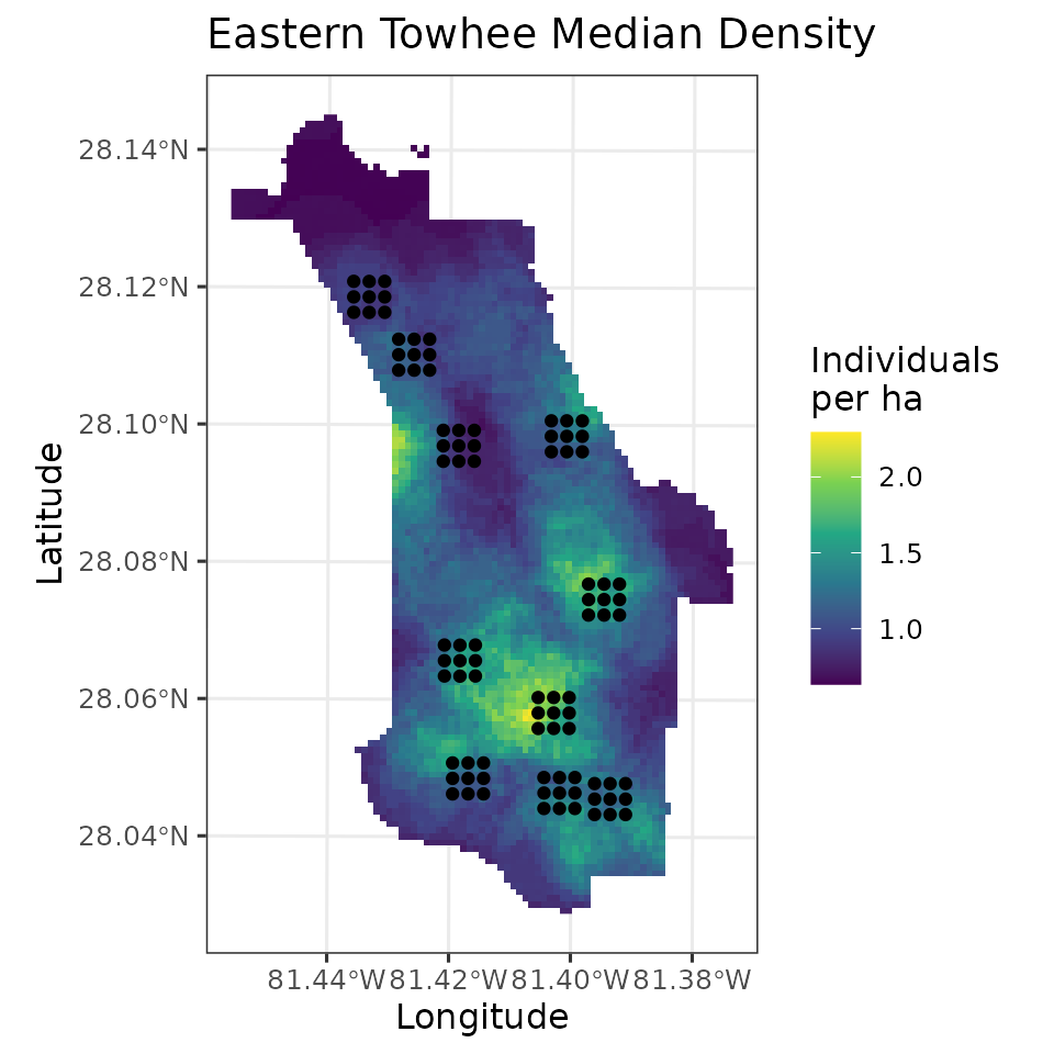
# Plot of 95% CI width
ggplot() +
geom_stars(data = coords.stars, aes(x = Easting, y = Northing, fill = mu.0.ci.width)) +
geom_sf(data = coords.sf) +
scale_fill_viridis_c(na.value = NA) +
theme_bw(base_size = 12) +
labs(fill = 'Individuals\nper ha', x = 'Longitude', y = 'Latitude',
title = 'Eastern Towhee Density 95% CI Width')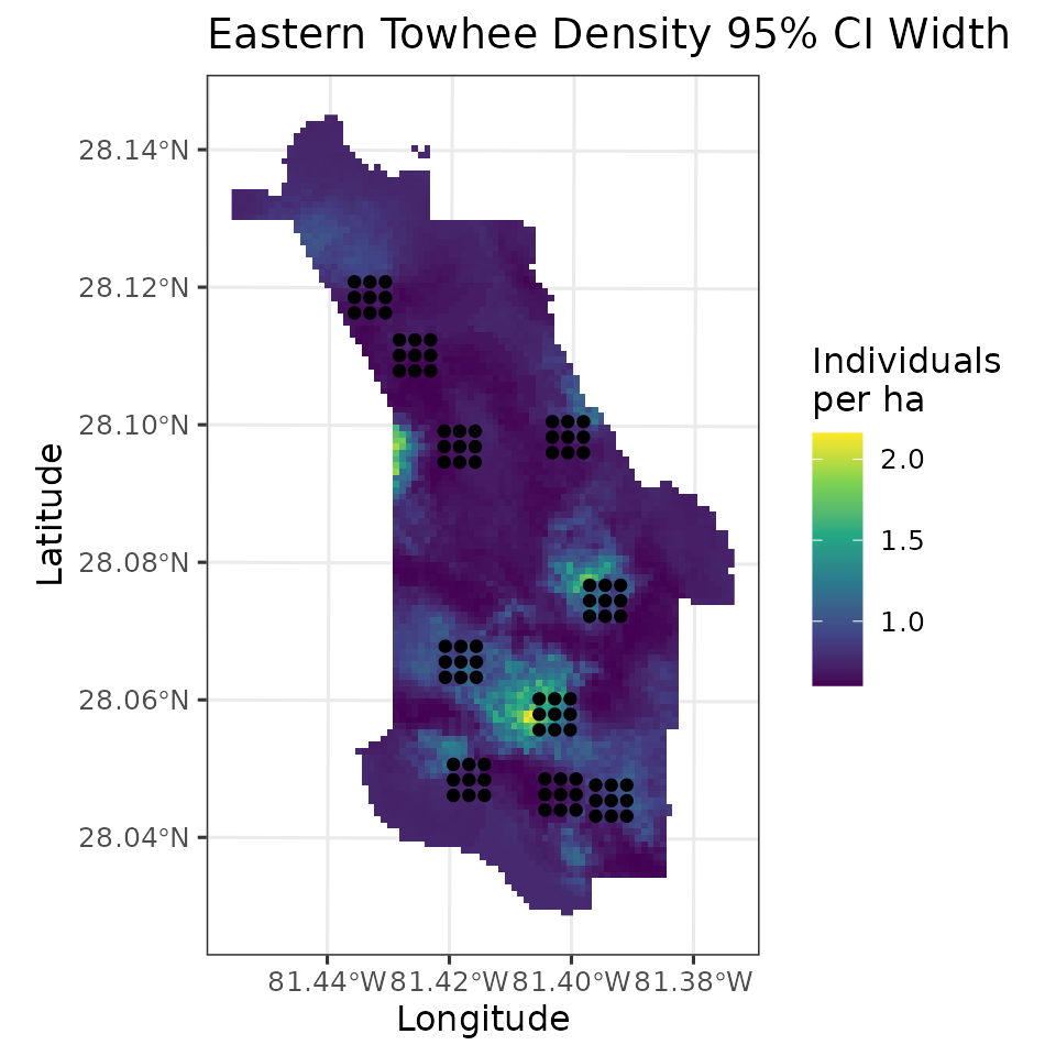
Single-species spatial HDS models
Basic model description
When working across large spatial domains, accounting for residual spatial autocorrelation in species distributions can often improve predictive performance of a model, leading to more accurate predictions of species abundance patterns (Guélat and Kéry 2018). We here extend the basic single-species HDS model to incorporate a spatial random effect that accounts for unexplained spatial variation in species abundance across a region of interest. Let \(\boldsymbol{s}_j\) denote the geographical coordinates of site \(j\) for \(j = 1, \dots, J\). In all spatially-explicit models, we include \(\boldsymbol{s}_j\) directly in the notation of spatially-indexed variables to indicate the model is spatially-explicit. More specifically, the expected abundance at site \(j\) with coordinates \(\boldsymbol{s}_j\), \(\mu(\boldsymbol{s}_j)\), now takes the form
\[\begin{equation} \text{log}(\mu(\boldsymbol{s}_j) = \boldsymbol{x}(\boldsymbol{s}_j)^{\top}\boldsymbol{\beta} + \text{w}(\boldsymbol{s}_j), \end{equation}\]
where \(\text{w}(\boldsymbol{s}_j)\) is a spatial random effect modeled with a Nearest Neighbor Gaussian Process (NNGP; Datta et al. (2016)). More specifically, we have
\[\begin{equation} \textbf{w}(\boldsymbol{s}) \sim N(\boldsymbol{0}, \boldsymbol{\tilde{\Sigma}}(\boldsymbol{s}, \boldsymbol{s}', \boldsymbol{\theta})), \end{equation}\]
where \(\boldsymbol{\tilde{\Sigma}}(\boldsymbol{s}, \boldsymbol{s}', \boldsymbol{\theta})\) is the NNGP-derived spatial covariance matrix that originates from the full \(J \times J\) covariance matrix \(\boldsymbol{\Sigma}(\boldsymbol{s}, \boldsymbol{s}', \boldsymbol{\theta})\) that is a function of the distances between any pair of site coordinates \(\boldsymbol{s}\) and \(\boldsymbol{s}'\) and a set of parameters \((\boldsymbol{\theta})\) that govern the spatial process. The vector \(\boldsymbol{\theta}\) is equal to \(\boldsymbol{\theta} = \{\sigma^2, \phi, \nu\}\), where \(\sigma^2\) is a spatial variance parameter, \(\phi\) is a spatial decay parameter, and \(\nu\) is a spatial smoothness parameter. \(\nu\) is only specified when using a Matern correlation function. The detection portion of the HDS model remains unchanged from the non-spatial model. The NNGP is a computationally efficient alternative to working with a full Gaussian process model, which is notoriously slow for even moderately large data sets. See Datta et al. (2016) and Finley et al. (2019) for complete statistical details on the NNGP.
Fitting single-species spatial HDS models with
spDS()
The function spDS() fits single-species spatial HDS
models.
spDS(abund.formula, det.formula, data, inits, priors, tuning,
cov.model = 'exponential', NNGP = TRUE,
n.neighbors = 15, search.type = 'cb',
n.batch, batch.length, accept.rate = 0.43, family = 'Poisson',
transect = 'line', det.func = 'halfnormal',
n.omp.threads = 1, verbose = TRUE,
n.report = 100, n.burn = round(.10 * n.batch * batch.length), n.thin = 1,
n.chains = 1, ...)The arguments to spDS() are very similar to those we saw
with DS(), with a few additional components. The abundance
(abund.formula) and detection (det.formula)
formulas, as well as the list of data (data), take the same
form as we saw in DS(), with random slopes and intercepts
allowed in both the abundance and detection models. Notice the
coords matrix in the data.EATO list of data.
We did not use this for DS() (except when making the map of
the predicted values), but specifying the spatial coordinates in
data is necessary for all spatially explicit models in
spAbundance.
abund.formula <- ~ scale(forest) + scale(grass)
det.formula <- ~ scale(wind)
str(dat.EATO) # coords is required for spDS()List of 5
$ y : num [1:90, 1:4] 0 0 0 0 0 0 0 0 0 0 ...
$ covs :'data.frame': 90 obs. of 4 variables:
..$ wind : int [1:90] 0 0 0 1 0 0 1 0 0 1 ...
..$ day : num [1:90] 132 132 132 132 132 132 132 132 132 129 ...
..$ forest: num [1:90] 0.18 0.0962 0.0577 0.1569 0.08 ...
..$ grass : num [1:90] 0.2 0.192 0.192 0.216 0.22 ...
$ dist.breaks: num [1:5] 0 0.025 0.05 0.1 0.25
$ offset : num 19.6
$ coords : num [1:90, 1:2] 458629 458879 459129 458629 458879 ...
..- attr(*, "dimnames")=List of 2
.. ..$ : NULL
.. ..$ : chr [1:2] "easting" "northing"The initial values (inits) are again specified in a
list. Valid tags for initial values now additionally include the
parameters associated with the spatial random effects. These include:
sigma.sq (spatial variance parameter), phi
(spatial decay parameter), w (the latent spatial random
effects at each site), and nu (spatial smoothness
parameter), where the latter is only specified if adopting a Matern
covariance function (i.e., cov.model = 'matern').
spAbundance supports four spatial covariance models
(exponential, spherical,
gaussian, and matern), which are specified in
the cov.model argument. Throughout this vignette, we will
use an exponential covariance model, which we often use as our default
covariance model when fitting spatially-explicit models and is commonly
used throughout ecology. To determine which covariance function to use,
we can fit models with the different covariance functions and compare
them using WAIC to select the best performing function. We will note
that the Matern covariance function has the additional spatial
smoothness parameter \(\nu\) and thus
can often be more flexible than the other functions. However, because we
need to estimate an additional parameter, this also tends to require
more data (i.e., a larger number of sites) than the other covariance
functions, and so we encourage use of the three simpler functions if
your data set is sparse. We note that model estimates are generally
fairly robust to the different covariance functions, although certain
functions may provide substantially better estimates depending on the
specific form of the underlying spatial autocorrelation in the data. For
example, the Gaussian covariance function is often useful for accounting
for spatial autocorrelation that is very smooth (i.e., long range
spatial dependence). See Chapter 2 in Banerjee,
Carlin, and Gelfand (2003) for a more thorough discussion of
these functions and their mathematical properties.
The default initial values for phi, and nu
are set to random values from the prior distribution, while the default
initial value for sigma.sq is set to a random value between
0.05 and 3. In all spatially-explicit models described in this vignette,
the spatial decay parameter phi is often the most sensitive
to initial values. In general, the spatial decay parameter will often
have poor mixing and take longer to converge than the rest of the
parameters in the model, so specifying an initial value that is
reasonably close to the resulting value can really help decrease run
times for complicated models. As an initial value for the spatial decay
parameter phi, we compute the mean distance between points
in our coordinates matrix and then set it equal to 3 divided by this
mean distance. When using an exponential covariance function, \(\frac{3}{\phi}\) is the effective range, or
the distance at which the residual spatial correlation between two sites
drops to 0.05 (Banerjee, Carlin, and Gelfand
2003). Thus our initial guess for this effective range is the
average distance between sites across the study region. As with all
other parameters, we generally recommend using the default initial
values for an initial model run, and if the model is taking a very long
time to converge you can rerun the model with initial values based on
the posterior means of estimated parameters from the initial model fit.
For the spatial variance parameter sigma.sq, we set the
initial value to 1. This corresponds to a moderate amount of spatial
variance. Further, we set the initial values of the latent spatial
random effects at each site to 0. The initial values for these random
effects has an extremely small influence on the model results, so we
generally recommend setting their initial values to 0 as we have done
here (this is also the default). However, if you are running your model
for a very long time and are seeing very slow convergence of the MCMC
chains, setting the initial values of the spatial random effects to the
mean estimates from a previous run of the model could help reach
convergence faster.
# Pair-wise distances between all sites
dist.mat <- dist(dat.EATO$coords)
# Exponential covariance model
cov.model <- 'exponential'
# Specify list of inits
inits.list <- list(beta = 0, alpha = 0, kappa = 1,
sigma.sq = 1, phi = 3 / mean(dist.mat),
w = rep(0, nrow(dat.EATO$y)),
N = apply(dat.EATO$y, 1, sum))The parameter NNGP is a logical value that specifies
whether we want to use an NNGP to fit the model. Currently, only
NNGP = TRUE is supported, but we may eventually add
functionality to fit full Gaussian Process models. The arguments
n.neighbors and search.type specify the number
of neighbors used in the NNGP and the nearest neighbor search algorithm,
respectively, to use for the NNGP model. Generally, the default values
of these arguments will be adequate. Datta et al.
(2016) showed that setting n.neighbors = 15 is
usually sufficient, although for certain data sets a good approximation
can be achieved with as few as five neighbors, which could substantially
decrease run time for the model. We generally recommend leaving
search.type = "cb", as this results in a fast code book
nearest neighbor search algorithm. However, details on when you may want
to change this are described in Finley, Datta,
and Banerjee (2020). We will run an NNGP model using the default
value for search.type and setting
n.neighbors = 15 (both the defaults).
NNGP <- TRUE
n.neighbors <- 15
search.type <- 'cb'Priors are again specified in a list in the argument
priors. We follow standard recommendations for prior
distributions from the spatial statistics literature (Banerjee, Carlin, and Gelfand 2003). We assume
an inverse gamma prior for the spatial variance parameter
sigma.sq (the tag of which is sigma.sq.ig),
and uniform priors for the spatial decay parameter phi and
smoothness parameter nu (if using the Matern correlation
function), with the associated tags phi.unif and
nu.unif. The hyperparameters of the inverse Gamma are
passed as a vector of length two, with the first and second elements
corresponding to the shape and scale, respectively. The lower and upper
bounds of the uniform distribution are passed as a two-element vector
for the uniform priors. We also allow users to restrict the spatial
variance further by specifying a uniform prior (with the tag
sigma.sq.unif), which can potentially be useful to place a
more informative prior on the spatial parameters. Generally, we use an
inverse-Gamma prior.
Note that the priors for the spatial parameters in a
spatially-explicit model must be at least weakly informative for the
model to converge (Banerjee, Carlin, and Gelfand
2003). For the inverse-Gamma prior on the spatial variance, we
typically set the shape parameter to 2 and the scale parameter equal to
our best guess of the spatial variance. The default prior hyperparameter
values for the spatial variance \(\sigma^2\) are a shape parameter of 2 and a
scale parameter of 1. This weakly informative prior suggests a prior
mean of 1 for the spatial variance, which is a moderately small amount
of spatial variation. Here we will use this default prior. For the
spatial decay parameter, our default approach is to set the lower and
upper bounds of the uniform prior based on the minimum and maximum
distances between sites in the data. More specifically, by default we
set the lower bound to 3 / max and the upper bound to
3 / min, where min and max are
the minimum and maximum distances between sites in the data set,
respectively. This equates to a vague prior that states the spatial
autocorrelation in the data could only exist between sites that are very
close together, or could span across the entire observed study area. If
additional information is known on the extent of the spatial
autocorrelation in the data, you may place more restrictive bounds on
the uniform prior, which would likely reduce the amount of time needed
for adequate mixing and convergence of the MCMC chains. Here we use this
default approach, but will explicitly set the values for
transparency.
min.dist <- min(dist.mat)
max.dist <- max(dist.mat)
priors <- list(alpha.normal = list(mean = 0, var = 100),
beta.normal = list(mean = 0, var = 100),
kappa.unif = c(0, 100),
sigma.sq.ig = c(2, 1),
phi.unif = c(3 / max.dist, 3 / min.dist))We again split our MCMC algorithm up into a set of batches and use an
adaptive sampler to adaptively tune the variances that we propose new
values from. We specify the initial tuning values again in the
tuning argument, and now need to add phi and
w to the parameters that must be tuned. Note that we do not
need to add sigma.sq, as this parameter can be sampled with
a more efficient approach (i.e., it’s full conditional distribution is
available in closed form).
tuning <- list(beta = 0.5, alpha = 0.5, kappa = 0.5, beta.star = 0.5,
w = 0.5, phi = 0.5)The argument n.omp.threads specifies the number of
threads to use for within-chain parallelization, while
verbose specifies whether or not to print the progress of
the sampler. As before, the argument n.report specifies the
interval to report the Metropolis-Hastings sampler acceptance rate.
Below we set n.report = 500, which will result in
information on the acceptance rate and tuning parameters every 500th
batch.
verbose <- TRUE
batch.length <- 25
n.batch <- 2000
# Total number of MCMC samples per chain
batch.length * n.batch[1] 50000
n.report <- 500
n.omp.threads <- 1We will use the same amount of burn-in and thinning as we did with
the non-spatial model, and we’ll also first fit a model with a Poisson
distribution for abundance. We next fit the model and summarize the
results using the summary() function. Recall that as
before, our data list contains an offset to convert the
estimates from individuals per point count to individuals per hectare.
As before, we set the det.func = 'halfnormal' to use a
half-normal detection function and set transect = 'point'
to indicate we are using data from circular surveys (i.e., point count
surveys).
n.burn <- 20000
n.thin <- 30
n.chains <- 3
# Approx. run time: 2 minutes
out.sp <- spDS(abund.formula = abund.formula,
det.formula = det.formula,
data = dat.EATO,
inits = inits.list,
priors = priors,
n.batch = n.batch,
batch.length = batch.length,
tuning = tuning,
cov.model = cov.model,
NNGP = NNGP,
n.neighbors = n.neighbors,
search.type = search.type,
n.omp.threads = n.omp.threads,
n.report = n.report,
family = 'Poisson',
det.func = 'halfnormal',
transect = 'point',
verbose = TRUE,
n.burn = n.burn,
n.thin = n.thin,
n.chains = n.chains)----------------------------------------
Preparing to run the model
----------------------------------------
----------------------------------------
Building the neighbor list
----------------------------------------
----------------------------------------
Building the neighbors of neighbors list
----------------------------------------
----------------------------------------
Model description
----------------------------------------
Spatial NNGP Poisson HDS model with 90 sites.
Samples per Chain: 50000 (2000 batches of length 25)
Burn-in: 20000
Thinning Rate: 30
Number of Chains: 3
Total Posterior Samples: 3000
Using the exponential spatial correlation model.
Using 15 nearest neighbors.
Source compiled with OpenMP support and model fit using 1 thread(s).
Adaptive Metropolis with target acceptance rate: 43.0
----------------------------------------
Chain 1
----------------------------------------
Sampling ...
Batch: 500 of 2000, 25.00%
Parameter Acceptance Tuning
beta[1] 44.0 0.05485
beta[2] 44.0 0.05166
beta[3] 32.0 0.05376
alpha[1] 60.0 0.07257
alpha[2] 32.0 0.09043
phi 20.0 0.84947
-------------------------------------------------
Batch: 1000 of 2000, 50.00%
Parameter Acceptance Tuning
beta[1] 48.0 0.05270
beta[2] 48.0 0.05166
beta[3] 36.0 0.05376
alpha[1] 44.0 0.08021
alpha[2] 48.0 0.08689
phi 40.0 0.88413
-------------------------------------------------
Batch: 1500 of 2000, 75.00%
Parameter Acceptance Tuning
beta[1] 32.0 0.04963
beta[2] 52.0 0.05063
beta[3] 40.0 0.05063
alpha[1] 40.0 0.07114
alpha[2] 48.0 0.09043
phi 36.0 0.81616
-------------------------------------------------
Batch: 2000 of 2000, 100.00%
----------------------------------------
Chain 2
----------------------------------------
Sampling ...
Batch: 500 of 2000, 25.00%
Parameter Acceptance Tuning
beta[1] 52.0 0.05709
beta[2] 40.0 0.05485
beta[3] 44.0 0.05596
alpha[1] 40.0 0.07257
alpha[2] 44.0 0.08864
phi 52.0 0.78416
-------------------------------------------------
Batch: 1000 of 2000, 50.00%
Parameter Acceptance Tuning
beta[1] 32.0 0.05709
beta[2] 48.0 0.04963
beta[3] 32.0 0.05270
alpha[1] 60.0 0.07862
alpha[2] 44.0 0.09226
phi 36.0 0.83265
-------------------------------------------------
Batch: 1500 of 2000, 75.00%
Parameter Acceptance Tuning
beta[1] 32.0 0.05376
beta[2] 36.0 0.05376
beta[3] 36.0 0.05166
alpha[1] 48.0 0.07404
alpha[2] 40.0 0.07862
phi 56.0 0.88413
-------------------------------------------------
Batch: 2000 of 2000, 100.00%
----------------------------------------
Chain 3
----------------------------------------
Sampling ...
Batch: 500 of 2000, 25.00%
Parameter Acceptance Tuning
beta[1] 40.0 0.06184
beta[2] 40.0 0.05063
beta[3] 32.0 0.05270
alpha[1] 32.0 0.07554
alpha[2] 52.0 0.08348
phi 36.0 0.70953
-------------------------------------------------
Batch: 1000 of 2000, 50.00%
Parameter Acceptance Tuning
beta[1] 44.0 0.05709
beta[2] 40.0 0.05596
beta[3] 32.0 0.05485
alpha[1] 28.0 0.07862
alpha[2] 36.0 0.08689
phi 60.0 0.80000
-------------------------------------------------
Batch: 1500 of 2000, 75.00%
Parameter Acceptance Tuning
beta[1] 20.0 0.05485
beta[2] 52.0 0.05376
beta[3] 60.0 0.05063
alpha[1] 40.0 0.07554
alpha[2] 36.0 0.08864
phi 56.0 0.86663
-------------------------------------------------
Batch: 2000 of 2000, 100.00%
summary(out.sp)
Call:
spDS(abund.formula = abund.formula, det.formula = det.formula,
    data = dat.EATO, inits = inits.list, priors = priors, tuning = tuning,
    cov.model = cov.model, NNGP = NNGP, n.neighbors = n.neighbors,
    search.type = search.type, n.batch = n.batch, batch.length = batch.length,
    family = "Poisson", transect = "point", det.func = "halfnormal",
    n.omp.threads = n.omp.threads, verbose = TRUE, n.report = n.report,
    n.burn = n.burn, n.thin = n.thin, n.chains = n.chains)

Samples per Chain: 50000
Burn-in: 20000
Thinning Rate: 30
Number of Chains: 3
Total Posterior Samples: 3000
Run Time (min): 1.634

Abundance (log scale):
                 Mean     SD    2.5%     50%  97.5%   Rhat ESS
(Intercept)    0.1021 0.2828 -0.4297  0.0949 0.7179 1.4272  60
scale(forest)  0.1414 0.1363 -0.1153  0.1428 0.4104 1.0079 249
scale(grass)  -0.0114 0.1439 -0.2843 -0.0144 0.2708 1.0226 262

Detection (log scale):
               Mean     SD    2.5%     50%   97.5%   Rhat ESS
(Intercept) -3.0890 0.0470 -3.1770 -3.0892 -2.9975 1.0214 345
scale(wind) -0.0471 0.0406 -0.1222 -0.0477  0.0343 1.0167 933

Spatial Covariance:
           Mean     SD   2.5%    50%  97.5%   Rhat ESS
sigma.sq 0.3404 0.1572 0.1427 0.3076 0.7266 1.0083 557
phi      0.0014 0.0012 0.0004 0.0010 0.0044 1.0157 361
Looking at the model summary we see adequate convergence of most
model parameters with the exception of the abundance intercept, so in a
complete analysis we would run this model longer to ensure all Rhat
values were less than 1.1. The summary() output looks the
same as what we saw previously, with the additional section titled
“Spatial Covariance”. There we see the estimate of the spatial variance
(sigma.sq) and spatial decay (phi) parameters.
The spatial variance is around 0.35, which indicates only a moderate
amount of spatial variability in abundance that is not explained by the
covariates. Interpretation of the spatial variance parameter can follow
interpretation of variance parameters in “regular” (i.e., unstructured)
random effect variances: when the variance is close to 0, that indicates
little support for inclusion of the spatial random effect. When the
variance is large, it indicates substantial support for the spatial
random effect. What indicates “large” vs. “small” isn’t necessarily
straightforward, and remember that we are working on the log scale. We
can also look at the magnitude of the spatial random effect estimates
themselves to give an indication as to how much residual spatial
autocorrelation there is in the abundance estimates. The posterior
samples for the spatial random effects are stored in the
w.samples tag of the resulting model fit list. Here we
calculate the means of the spatial random effects and plot a histogram
of their values.
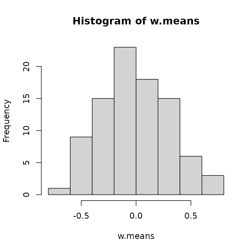
We see most values are clustered around 0, but that there are a few fairly large positive and negative values.
Posterior predictive checks
Posterior predictive checks proceed exactly as before using the
ppcAbund() function.
Call:
ppcAbund(object = out.sp, fit.stat = "freeman-tukey", group = 1)

Samples per Chain: 50000
Burn-in: 20000
Thinning Rate: 30
Number of Chains: 3
Total Posterior Samples: 3000

Bayesian p-value:  0.5443
Fit statistic:  freeman-tukey
Model selection using WAIC
We next compare the spatial HDS model to the non-spatial HDS model we
fit previously (stored in out).
# Non-spatial
waicAbund(out)
N.max not specified. Setting upper index of integration of N to 10 plus
the largest estimated abundance value at each site in object$N.samples elpd pD WAIC
-255.728227 5.173769 521.803993
# Spatial
waicAbund(out.sp)
N.max not specified. Setting upper index of integration of N to 10 plus
the largest estimated abundance value at each site in object$N.samples elpd pD WAIC
-240.75652 13.27545 508.06395 Here we see fairly substantial improvement in the WAIC for the spatial model compared to the non-spatial model (i.e., WAIC is lower for the spatial model).
Prediction
We can similarly predict across a region of interest using the
predict() function as we saw with the non-spatial HDS
model. Here we again generate predictions across a 1ha grid of the
Disney Wilderness Preserve. The primary arguments for prediction here
are identical to those we saw for the non-spatial model, with the
addition of the coords argument to specify the spatial
coordinates of the prediction locations. These are necessary to generate
the predictions of the spatial random effects. We use the same design
matrix that we previously formed for the non-spatial predictions
(X.0), which contains the covariate values standardized by
the values used when we fit the model. There are also arguments for
parallelization (n.omp.threads), reporting sampler progress
(verbose and n.report), and predicting without
the spatial random effects (include.sp). We generally only
recommend setting include.sp = FALSE when generating
predictions for a marginal probability plot (see the N-mixture
model vignette for an example of this).
# Look at the prediction data set again
str(neonPredData)
'data.frame': 4838 obs. of 4 variables:
$ forest : num 0.0208 0.0196 0.0196 0.02 0.0192 ...
$ grass : num 0.188 0.176 0.176 0.18 0.192 ...
$ easting : num 456756 456856 456456 456556 456656 ...
$ northing: num 3113309 3113309 3113209 3113209 3113209 ...
# Coordinates are needed for prediction with spatial HDS models
coords.0 <- neonPredData[, c('easting', 'northing')]
out.sp.pred <- predict(out.sp, X.0, coords = coords.0, n.report = 400)
----------------------------------------
Prediction description
----------------------------------------
NNGP spatial abundance model with 90 observations.
Number of covariates 3 (including intercept if specified).
Using the exponential spatial correlation model.
Using 15 nearest neighbors.
Number of MCMC samples 3000.
Predicting at 4838 locations.
Source compiled with OpenMP support and model fit using 1 threads.
-------------------------------------------------
Predicting
-------------------------------------------------
Location: 400 of 4838, 8.27%
Location: 800 of 4838, 16.54%
Location: 1200 of 4838, 24.80%
Location: 1600 of 4838, 33.07%
Location: 2000 of 4838, 41.34%
Location: 2400 of 4838, 49.61%
Location: 2800 of 4838, 57.88%
Location: 3200 of 4838, 66.14%
Location: 3600 of 4838, 74.41%
Location: 4000 of 4838, 82.68%
Location: 4400 of 4838, 90.95%
Location: 4800 of 4838, 99.21%
Location: 4838 of 4838, 100.00%
Generating latent abundance state
mu.0.quants <- apply(out.sp.pred$mu.0.samples, 2, quantile, c(0.025, 0.5, 0.975))
plot.df <- data.frame(Easting = neonPredData$easting,
                      Northing = neonPredData$northing,
                      mu.0.med = mu.0.quants[2, ],
                      mu.0.ci.width = mu.0.quants[3, ] - mu.0.quants[1, ])
coords.stars <- st_as_stars(plot.df, crs = st_crs(32617))
coords.sf <- st_as_sf(as.data.frame(dat.EATO$coords), coords = c('easting', 'northing'),
                      crs = st_crs(32617))
# Plot of median estimate
ggplot() +
  geom_stars(data = coords.stars, aes(x = Easting, y = Northing, fill = mu.0.med)) +
  geom_sf(data = coords.sf) +
  scale_fill_viridis_c(na.value = NA) +
  theme_bw(base_size = 14) +
  labs(fill = 'Individuals\nper ha', x = 'Longitude', y = 'Latitude',
       title = 'Eastern Towhee Median Density')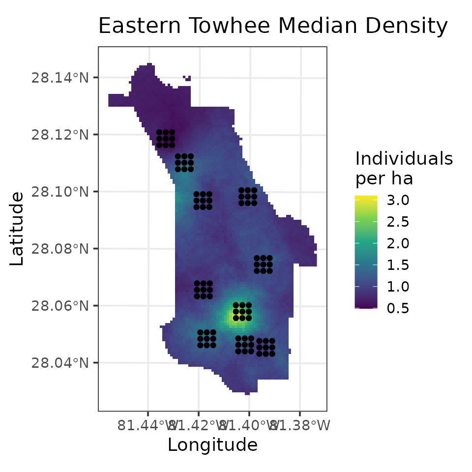
# Plot of 95% CI width
ggplot() +
  geom_stars(data = coords.stars, aes(x = Easting, y = Northing, fill = mu.0.ci.width)) +
  geom_sf(data = coords.sf) +
  scale_fill_viridis_c(na.value = NA) +
  theme_bw(base_size = 14) +
  labs(fill = 'Individuals\nper ha', x = 'Longitude', y = 'Latitude',
       title = 'Eastern Towhee Density 95% CI Width')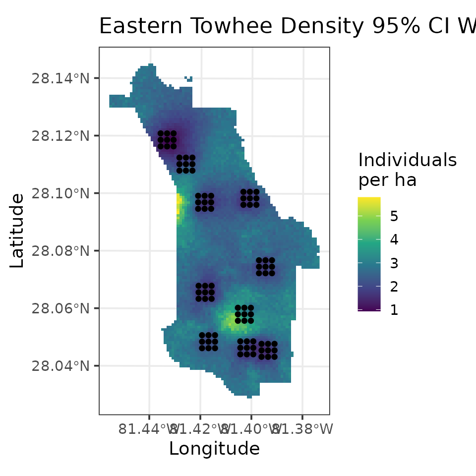
There are some interesting differences between the predictions of the spatial and non-spatial model, which we’ll leave to you to explore if you desire. Looking at the predictions of the spatial model, we immediately see two things: (1) the uncertainty is substantially larger than that of the non-spatial model; and (2) the uncertainty generally increases as one gets farther away from the observed locations. The latter point is a common phenomena we will observe when fitting any spatial model, and the degree to which the uncertainty increases as one gets farther away from sampled locations will depend on the estimated effective spatial range.
Multi-species HDS models
Basic model description
Now consider the case where distance sampling data, \(\boldsymbol{y}_{i, j}\), are collected for multiple species \(i = 1, \dots, I\) at each survey location \(j\). We are now interested in estimating the abundance of each species \(i\) at each location \(j\), denoted as \(N_{i, j}\). We model \(N_{i, j}\) analogous to the single-species HDS model, with expected abundance now varying by species and site according to
\[\begin{equation}\label{mu-msDS} \text{log}(\mu_{i, j}) = \boldsymbol{x}_j^\top\boldsymbol{\beta}_i, \end{equation}\]
where \(\boldsymbol{\beta}_i\) are the species-specific effects of covariates \(\boldsymbol{x}_j\) (including an intercept). When \(N_i(\boldsymbol{s}_j)\) is modeled using a negative binomial distribution, we estimate a separate dispersion parameter \(\kappa_i\) for each species. We model \(\boldsymbol{\beta}_i\) as random effects arising from a common, community-level normal distribution, which leads to increased precision of species-specific effects compared to single-species models (Sollmann et al. 2016). For example, the species-specific abundance intercept \(\beta_{0, i}\) is modeled according to
\[\begin{equation}\label{betaComm} \beta_{0, i} \sim \text{Normal}(\mu_{\beta_0}, \tau^2_{\beta_0}), \end{equation}\]
where \(\mu_{\beta_0}\) is the community-level abundance intercept, and \(\tau^2_{\beta_0}\) is the variance of the intercept across all \(I\) species. The observation portion of the multi-species HDS model is identical to the single-species model, with all parameters indexed by species, and the species-specific coefficients \(\boldsymbol{\alpha}_i\) modeled hierarchically analogous to the species-specific abundance coefficients just described.
We assign normal priors to the community-level abundance (\(\boldsymbol{\mu}_{\beta}\)) and detection (\(\boldsymbol{\mu}_{\alpha}\)) mean parameters and inverse-Gamma priors to the community-level variance parameters (\(\boldsymbol{\tau^2}_{\beta}\) and \(\boldsymbol{\tau^2}_{\alpha}\)). We give independent uniform priors to each of the species-specific negative binomial dispersion parameters \(\kappa_i\).
Fitting multi-species HDS models with msDS()
spAbundance uses nearly identical syntax for fitting
multi-species HDS models as it does for single-species models and
provides the same functionality for posterior predictive checks, model
assessment and selection using WAIC, and prediction. The
msDS() function fits the multi-species HDS model first
introduced by Sollmann et al. (2016).
msDS() has the following syntax
msDS(abund.formula, det.formula, data, inits, priors,
     tuning, n.batch, batch.length, accept.rate = 0.43,
     family = 'Poisson', transect = 'line', det.func = 'halfnormal',
     n.omp.threads = 1, verbose = TRUE, n.report = 100,
     n.burn = round(.10 * n.batch * batch.length), n.thin = 1,
     n.chains = 1, ...)
Notice these are the exact same arguments we saw with
DS(). We will now model the entire group of 16 bird species
contained in the neonDWP data set instead of just focusing
on EATO.
# Recall the structure of the full data set
str(neonDWP)
List of 5
$ y : num [1:16, 1:90, 1:4] 0 0 0 0 0 0 1 0 0 0 ...
..- attr(*, "dimnames")=List of 3
.. ..$ : chr [1:16] "EATO" "EAME" "AMCR" "BACS" ...
.. ..$ : NULL
.. ..$ : NULL
$ covs :'data.frame': 90 obs. of 4 variables:
..$ wind : int [1:90] 0 0 0 1 0 0 1 0 0 1 ...
..$ day : num [1:90] 132 132 132 132 132 132 132 132 132 129 ...
..$ forest: num [1:90] 0.18 0.0962 0.0577 0.1569 0.08 ...
..$ grass : num [1:90] 0.2 0.192 0.192 0.216 0.22 ...
$ dist.breaks: num [1:5] 0 0.025 0.05 0.1 0.25
$ offset : num 19.6
$ coords : num [1:90, 1:2] 458629 458879 459129 458629 458879 ...
..- attr(*, "dimnames")=List of 2
.. ..$ : NULL
.. ..$ : chr [1:2] "easting" "northing"For multi-species models, the multi-species detection-nondetection
data y is now a three-dimensional array with dimensions
corresponding to species, sites, and replicates. This is how the data
are provided in the neonDWP object, so we don’t need to do
any additional preparations. For guidance on preparing raw data into
such a three-dimensional array format, please see this
vignette on the spOccupancy website. The vignette
provides guidance for fitting multi-species models in
spOccupancy, but the format for spAbundance is
exactly the same and all the same guidance applies here. We will model
abundance and detection for all species using the same covariates as
before.
Next we specify the initial values in inits. For
multi-species HDS models, we supply initial values for community-level
and species-level parameters. In msDS(), we will supply
initial values for the following parameters: alpha.comm
(community-level detection coefficients), beta.comm
(community-level abundance coefficients), alpha
(species-level detection coefficients), beta (species-level
abundance coefficients), tau.sq.beta (community-level
abundance variance parameters), tau.sq.alpha
(community-level detection variance parameters), N (latent
abundance values for all species), kappa (species-level
negative binomial overdispersion parameters), sigma.sq.mu
(random effect variances for abundance), and sigma.sq.p
(random effect variances for detection). These are all specified in a
single list. Initial values for community-level parameters (including
the random effect variances) are either vectors of length corresponding
to the number of community-level detection or abundance parameters in
the model (including the intercepts) or a single value if all parameters
are assigned the same initial values. Initial values for species level
parameters are either matrices with the number of rows indicating the
number of species, and each column corresponding to a different
regression parameter, or a single value if the same initial value is
used for all species and parameters. Initial values for
kappa is similarly either a single value that is assumed to
be the same for all species, or a vector with a specific initial value
for each species. The initial values for the latent abundance matrix are
specified as a matrix with \(I\) rows
corresponding to the number of species and \(J\) columns corresponding to the number of
sites.
# Number of species
n.sp <- dim(neonDWP$y)[1]
ms.inits <- list(alpha.comm = 0,
beta.comm = 0,
beta = 0,
alpha = 0,
tau.sq.beta = 1,
kappa = 1,
tau.sq.alpha = 1,
sigma.sq.mu = 0.5,
N = apply(neonDWP$y, c(1, 2), sum, na.rm = TRUE))In multi-species models, we specify priors on the community-level
coefficients (or hyperparameters) rather than the species-level effects,
with the exception that we still assign uniform priors for the negative
binomial overdispersion parameter. For nonspatial models, these priors
are specified with the following tags: beta.comm.normal
(normal prior on the community-level abundance mean effects),
alpha.comm.normal (normal prior on the community-level
detection mean effects), tau.sq.beta.ig (inverse-Gamma
prior on the community-level abundance variance parameters),
tau.sq.alpha.ig (inverse-Gamma prior on the community-level
detection variance parameters), sigma.sq.mu.ig
(inverse-Gamma prior on the abundance random effect variances),
sigma.sq.p.ig (inverse-Gamma prior on the detection random
effect variances), kappa.unif (uniform prior on the
species-specific overdispersion parameters). For all parameters except
the species-specific overdispersion parameters, each tag consists of a
list with elements corresponding to the mean and variance for normal
priors and scale and shape for inverse-Gamma priors. Values can be
specified individually for each parameter or as a single value if the
same prior is assigned to all parameters of a given type. For the
species-specific overdispersion parameters, the prior is specified as a
list with two elements representing the lower and upper bound of the
uniform distribution, where each of the elements can be a single value
if the same prior is used for all species, or a vector of values for
each species if specifying a different prior for each species.
By default, we set the prior hyperparameter values for the
community-level means to a mean of 0 and a variance of 100. Below we
specify these priors explicitly. For the community-level variance
parameters, by default we set the scale and shape parameters to 0.1
following the recommendations of (Lunn et al.
2013), which results in a weakly informative prior on the
community-level variances. This may lead to shrinkage of the
community-level variance towards zero under certain circumstances so
that all species will have fairly similar values for the
species-specific covariate effect (Gelman
2006), although we have found multi-species models to be
relatively robust to this prior specification. We are in the process of
implementing half-Cauchy and half-t priors for the variance parameters
in all multi-species models in spAbundance (and
spOccupancy), which generally result in less shrinkage
toward zero than the inverse-Gamma (Gelman
2006). For the negative binomial overdispersion parameters, we by
default use a lower bound of 0 and upper bound of 100 for the uniform
priors for each species, as we did in the single-species (univariate)
models. Below we explicitly set these default prior values for our
example.
ms.priors <- list(beta.comm.normal = list(mean = 0, var = 100),
alpha.comm.normal = list(mean = 0, var = 100),
tau.sq.beta.ig = list(a = 0.1, b = 0.1),
tau.sq.alpha.ig = list(a = 0.1, b = 0.1),
kappa.unif = list(a = 0, b = 100))As before, we will fit a model with a Poisson distribution for
abundance (family = 'Poisson'), specify that we are using
point count data (transect = 'point'), and use a
half-normal detection function (det.func = 'halfnormal').
All that’s now left to do is specify the number of threads to use
(n.omp.threads), the number of MCMC samples (which we do by
specifying the number of batches n.batch and batch length
batch.length), the initial tuning variances
(tuning), the amount of samples to discard as burn-in
(n.burn), the thinning rate (n.thin), and
arguments to control the display of sampler progress
(verbose, n.report). Note for the tuning
variances, we do not need to specify initial tuning values for any of
the community-level parameters, as those parameters can be sampled with
an efficient Gibbs update.
# Specify initial tuning values
ms.tuning <- list(beta = 0.3, alpha = 0.3, beta.star = 0.5, kappa = 0.5)
# Approx. run time: 6 min
out.ms <- msDS(abund.formula = abund.formula,
det.formula = det.formula,
data = neonDWP,
inits = ms.inits,
n.batch = 2000,
tuning = ms.tuning,
batch.length = 25,
priors = ms.priors,
n.omp.threads = 1,
family = 'Poisson',
det.func = 'halfnormal',
transect = 'point',
verbose = TRUE,
n.report = 500,
n.burn = 20000,
n.thin = 30,
n.chains = 3)----------------------------------------
Preparing to run the model
----------------------------------------
----------------------------------------
Model description
----------------------------------------
Multi-species Poisson HDS model with 90 sites and 16 species.
Samples per Chain: 50000 (2000 batches of length 25)
Burn-in: 20000
Thinning Rate: 30
Number of Chains: 3
Total Posterior Samples: 3000
Source compiled with OpenMP support and model fit using 1 thread(s).
Adaptive Metropolis with target acceptance rate: 43.0
----------------------------------------
Chain 1
----------------------------------------
Sampling ...
Batch: 500 of 2000, 25.00%
Species Parameter Acceptance Tuning
1 beta[1] 48.0 0.05319
1 alpha[1] 40.0 0.07472
2 beta[1] 44.0 0.11147
2 alpha[1] 64.0 0.11372
3 beta[1] 44.0 0.46118
3 alpha[1] 48.0 0.32825
4 beta[1] 36.0 0.11372
4 alpha[1] 24.0 0.12076
5 beta[1] 40.0 0.17308
5 alpha[1] 44.0 0.14171
6 beta[1] 68.0 0.27418
6 alpha[1] 44.0 0.25821
7 beta[1] 28.0 0.31538
7 alpha[1] 64.0 0.29701
8 beta[1] 36.0 0.12822
8 alpha[1] 48.0 0.14171
9 beta[1] 48.0 0.15047
9 alpha[1] 44.0 0.16966
10 beta[1] 36.0 0.21141
10 alpha[1] 24.0 0.15351
11 beta[1] 60.0 0.11837
11 alpha[1] 40.0 0.10290
12 beta[1] 56.0 0.32175
12 alpha[1] 56.0 0.23364
13 beta[1] 48.0 0.22003
13 alpha[1] 36.0 0.17658
14 beta[1] 40.0 0.19515
14 alpha[1] 44.0 0.15047
15 beta[1] 32.0 0.39299
15 alpha[1] 40.0 0.31538
16 beta[1] 48.0 0.22003
16 alpha[1] 16.0 0.20722
-------------------------------------------------
Batch: 1000 of 2000, 50.00%
Species Parameter Acceptance Tuning
1 beta[1] 64.0 0.05536
1 alpha[1] 56.0 0.07777
2 beta[1] 48.0 0.11147
2 alpha[1] 44.0 0.11837
3 beta[1] 44.0 0.48969
3 alpha[1] 32.0 0.34165
4 beta[1] 12.0 0.12822
4 alpha[1] 32.0 0.12822
5 beta[1] 44.0 0.15661
5 alpha[1] 48.0 0.13081
6 beta[1] 48.0 0.24809
6 alpha[1] 40.0 0.24318
7 beta[1] 36.0 0.31538
7 alpha[1] 40.0 0.26875
8 beta[1] 36.0 0.13081
8 alpha[1] 44.0 0.12569
9 beta[1] 48.0 0.17308
9 alpha[1] 44.0 0.19129
10 beta[1] 36.0 0.21141
10 alpha[1] 40.0 0.16966
11 beta[1] 60.0 0.13346
11 alpha[1] 44.0 0.11372
12 beta[1] 36.0 0.31538
12 alpha[1] 48.0 0.24318
13 beta[1] 32.0 0.22448
13 alpha[1] 36.0 0.20312
14 beta[1] 40.0 0.19129
14 alpha[1] 32.0 0.15351
15 beta[1] 44.0 0.40903
15 alpha[1] 48.0 0.32175
16 beta[1] 44.0 0.22003
16 alpha[1] 44.0 0.21141
-------------------------------------------------
Batch: 1500 of 2000, 75.00%
Species Parameter Acceptance Tuning
1 beta[1] 56.0 0.05761
1 alpha[1] 56.0 0.07777
2 beta[1] 44.0 0.11372
2 alpha[1] 32.0 0.11602
3 beta[1] 20.0 0.45205
3 alpha[1] 52.0 0.33488
4 beta[1] 56.0 0.11837
4 alpha[1] 68.0 0.11837
5 beta[1] 36.0 0.15047
5 alpha[1] 36.0 0.14457
6 beta[1] 52.0 0.25821
6 alpha[1] 52.0 0.25310
7 beta[1] 64.0 0.26343
7 alpha[1] 40.0 0.29113
8 beta[1] 44.0 0.12822
8 alpha[1] 60.0 0.13081
9 beta[1] 36.0 0.16301
9 alpha[1] 48.0 0.17308
10 beta[1] 32.0 0.19910
10 alpha[1] 56.0 0.15978
11 beta[1] 32.0 0.12822
11 alpha[1] 64.0 0.11147
12 beta[1] 48.0 0.30914
12 alpha[1] 48.0 0.23836
13 beta[1] 44.0 0.24318
13 alpha[1] 24.0 0.18750
14 beta[1] 32.0 0.20312
14 alpha[1] 48.0 0.14457
15 beta[1] 40.0 0.38521
15 alpha[1] 64.0 0.29113
16 beta[1] 40.0 0.23364
16 alpha[1] 24.0 0.20312
-------------------------------------------------
Batch: 2000 of 2000, 100.00%
----------------------------------------
Chain 2
----------------------------------------
Sampling ...
Batch: 500 of 2000, 25.00%
Species Parameter Acceptance Tuning
1 beta[1] 36.0 0.05426
1 alpha[1] 40.0 0.07037
2 beta[1] 40.0 0.10710
2 alpha[1] 24.0 0.10290
3 beta[1] 24.0 0.41729
3 alpha[1] 28.0 0.27418
4 beta[1] 44.0 0.12822
4 alpha[1] 44.0 0.13890
5 beta[1] 44.0 0.17308
5 alpha[1] 44.0 0.13890
6 beta[1] 28.0 0.25821
6 alpha[1] 36.0 0.24318
7 beta[1] 36.0 0.31538
7 alpha[1] 60.0 0.26343
8 beta[1] 36.0 0.13890
8 alpha[1] 36.0 0.12076
9 beta[1] 68.0 0.15978
9 alpha[1] 28.0 0.15661
10 beta[1] 40.0 0.19129
10 alpha[1] 28.0 0.14171
11 beta[1] 48.0 0.13346
11 alpha[1] 36.0 0.10927
12 beta[1] 40.0 0.29113
12 alpha[1] 20.0 0.23364
13 beta[1] 16.0 0.22003
13 alpha[1] 52.0 0.17308
14 beta[1] 60.0 0.19910
14 alpha[1] 36.0 0.14457
15 beta[1] 52.0 0.36277
15 alpha[1] 8.0 0.27972
16 beta[1] 44.0 0.25310
16 alpha[1] 24.0 0.19910
-------------------------------------------------
Batch: 1000 of 2000, 50.00%
Species Parameter Acceptance Tuning
1 beta[1] 40.0 0.06241
1 alpha[1] 52.0 0.07934
2 beta[1] 48.0 0.10710
2 alpha[1] 36.0 0.11147
3 beta[1] 36.0 0.37758
3 alpha[1] 44.0 0.29701
4 beta[1] 40.0 0.11602
4 alpha[1] 40.0 0.12076
5 beta[1] 28.0 0.15047
5 alpha[1] 36.0 0.13081
6 beta[1] 48.0 0.25821
6 alpha[1] 52.0 0.24809
7 beta[1] 32.0 0.25821
7 alpha[1] 28.0 0.24809
8 beta[1] 36.0 0.13615
8 alpha[1] 32.0 0.13346
9 beta[1] 40.0 0.15978
9 alpha[1] 56.0 0.18750
10 beta[1] 44.0 0.19129
10 alpha[1] 32.0 0.13890
11 beta[1] 52.0 0.12320
11 alpha[1] 52.0 0.10710
12 beta[1] 36.0 0.29701
12 alpha[1] 60.0 0.24318
13 beta[1] 40.0 0.22003
13 alpha[1] 20.0 0.17658
14 beta[1] 44.0 0.19515
14 alpha[1] 48.0 0.15661
15 beta[1] 48.0 0.41729
15 alpha[1] 36.0 0.30914
16 beta[1] 52.0 0.24318
16 alpha[1] 56.0 0.20722
-------------------------------------------------
Batch: 1500 of 2000, 75.00%
Species Parameter Acceptance Tuning
1 beta[1] 36.0 0.05426
1 alpha[1] 20.0 0.07934
2 beta[1] 32.0 0.11147
2 alpha[1] 56.0 0.11602
3 beta[1] 44.0 0.40903
3 alpha[1] 36.0 0.32825
4 beta[1] 44.0 0.10927
4 alpha[1] 44.0 0.12320
5 beta[1] 64.0 0.15661
5 alpha[1] 48.0 0.14749
6 beta[1] 44.0 0.25821
6 alpha[1] 44.0 0.24318
7 beta[1] 44.0 0.23364
7 alpha[1] 32.0 0.25821
8 beta[1] 32.0 0.11837
8 alpha[1] 40.0 0.12822
9 beta[1] 24.0 0.17658
9 alpha[1] 40.0 0.18015
10 beta[1] 40.0 0.19910
10 alpha[1] 20.0 0.15351
11 beta[1] 52.0 0.11372
11 alpha[1] 24.0 0.10290
12 beta[1] 48.0 0.30914
12 alpha[1] 44.0 0.21568
13 beta[1] 52.0 0.22448
13 alpha[1] 40.0 0.19129
14 beta[1] 40.0 0.19515
14 alpha[1] 36.0 0.15047
15 beta[1] 68.0 0.40903
15 alpha[1] 40.0 0.30302
16 beta[1] 40.0 0.24809
16 alpha[1] 40.0 0.19129
-------------------------------------------------
Batch: 2000 of 2000, 100.00%
----------------------------------------
Chain 3
----------------------------------------
Sampling ...
Batch: 500 of 2000, 25.00%
Species Parameter Acceptance Tuning
1 beta[1] 36.0 0.05009
1 alpha[1] 40.0 0.07623
2 beta[1] 52.0 0.10927
2 alpha[1] 32.0 0.11147
3 beta[1] 56.0 0.46118
3 alpha[1] 36.0 0.30914
4 beta[1] 56.0 0.12569
4 alpha[1] 52.0 0.12569
5 beta[1] 52.0 0.15978
5 alpha[1] 36.0 0.13081
6 beta[1] 52.0 0.25310
6 alpha[1] 28.0 0.24809
7 beta[1] 52.0 0.29701
7 alpha[1] 44.0 0.26875
8 beta[1] 48.0 0.14171
8 alpha[1] 48.0 0.13081
9 beta[1] 52.0 0.18379
9 alpha[1] 52.0 0.16630
10 beta[1] 56.0 0.19515
10 alpha[1] 60.0 0.15661
11 beta[1] 40.0 0.14171
11 alpha[1] 32.0 0.10498
12 beta[1] 48.0 0.33488
12 alpha[1] 48.0 0.23364
13 beta[1] 72.0 0.22003
13 alpha[1] 48.0 0.20722
14 beta[1] 44.0 0.21141
14 alpha[1] 24.0 0.15978
15 beta[1] 48.0 0.40093
15 alpha[1] 48.0 0.29701
16 beta[1] 40.0 0.22448
16 alpha[1] 20.0 0.20312
-------------------------------------------------
Batch: 1000 of 2000, 50.00%
Species Parameter Acceptance Tuning
1 beta[1] 48.0 0.05426
1 alpha[1] 36.0 0.07623
2 beta[1] 44.0 0.11372
2 alpha[1] 48.0 0.11837
3 beta[1] 32.0 0.45205
3 alpha[1] 44.0 0.33488
4 beta[1] 36.0 0.11837
4 alpha[1] 36.0 0.12320
5 beta[1] 28.0 0.16966
5 alpha[1] 48.0 0.14171
6 beta[1] 20.0 0.22003
6 alpha[1] 36.0 0.23836
7 beta[1] 40.0 0.37010
7 alpha[1] 44.0 0.32825
8 beta[1] 60.0 0.12569
8 alpha[1] 48.0 0.12822
9 beta[1] 44.0 0.18379
9 alpha[1] 60.0 0.18379
10 beta[1] 52.0 0.19910
10 alpha[1] 56.0 0.17658
11 beta[1] 44.0 0.12822
11 alpha[1] 40.0 0.10498
12 beta[1] 32.0 0.29701
12 alpha[1] 28.0 0.20722
13 beta[1] 64.0 0.23364
13 alpha[1] 40.0 0.18015
14 beta[1] 28.0 0.21141
14 alpha[1] 44.0 0.16630
15 beta[1] 40.0 0.40903
15 alpha[1] 60.0 0.29701
16 beta[1] 28.0 0.20312
16 alpha[1] 48.0 0.22003
-------------------------------------------------
Batch: 1500 of 2000, 75.00%
Species Parameter Acceptance Tuning
1 beta[1] 36.0 0.05213
1 alpha[1] 40.0 0.07623
2 beta[1] 44.0 0.10710
2 alpha[1] 32.0 0.13081
3 beta[1] 36.0 0.41729
3 alpha[1] 52.0 0.31538
4 beta[1] 60.0 0.11837
4 alpha[1] 20.0 0.12076
5 beta[1] 28.0 0.16301
5 alpha[1] 40.0 0.14457
6 beta[1] 32.0 0.26343
6 alpha[1] 44.0 0.25821
7 beta[1] 40.0 0.27972
7 alpha[1] 40.0 0.27418
8 beta[1] 60.0 0.13346
8 alpha[1] 28.0 0.12076
9 beta[1] 32.0 0.16301
9 alpha[1] 36.0 0.17658
10 beta[1] 60.0 0.20722
10 alpha[1] 56.0 0.15351
11 beta[1] 28.0 0.12822
11 alpha[1] 48.0 0.11147
12 beta[1] 68.0 0.29701
12 alpha[1] 64.0 0.23364
13 beta[1] 56.0 0.20312
13 alpha[1] 52.0 0.17658
14 beta[1] 48.0 0.23364
14 alpha[1] 44.0 0.17658
15 beta[1] 32.0 0.37758
15 alpha[1] 32.0 0.29701
16 beta[1] 48.0 0.19910
16 alpha[1] 48.0 0.19515
-------------------------------------------------
Batch: 2000 of 2000, 100.00%The resulting object out.ms is a list of class
msDS consisting primarily of posterior samples of all
community and species-level parameters, as well as some additional
objects that are used for summaries, prediction, and model fit
evaluation. We can display a nice summary of these results using the
summary() function as before. For multi-species objects,
when using summary we need to specify the level of parameters we want to
summarize. We do this using the argument level, which takes
values community, species, or
both to print results for community-level parameters,
species-level parameters, or all parameters. By default,
level is set to both to display both species
and community-level parameters.
summary(out.ms)
Call:
msDS(abund.formula = abund.formula, det.formula = det.formula,
data = neonDWP, inits = ms.inits, priors = ms.priors, tuning = ms.tuning,
n.batch = 2000, batch.length = 25, family = "Poisson", transect = "point",
det.func = "halfnormal", n.omp.threads = 1, verbose = TRUE,
n.report = 500, n.burn = 20000, n.thin = 30, n.chains = 3)
Samples per Chain: 50000
Burn-in: 20000
Thinning Rate: 30
Number of Chains: 3
Total Posterior Samples: 3000
Run Time (min): 5.9223
----------------------------------------
Community Level
----------------------------------------
Abundance Means (log scale):
Mean SD 2.5% 50% 97.5% Rhat ESS
(Intercept) -2.3951 0.3251 -3.0359 -2.3854 -1.7708 1.0020 3000
scale(forest) -0.0488 0.0937 -0.2423 -0.0445 0.1296 1.0084 1820
scale(grass) 0.0589 0.1155 -0.1658 0.0576 0.2905 1.0113 2527
Abundance Variances (log scale):
Mean SD 2.5% 50% 97.5% Rhat ESS
(Intercept) 1.5595 0.7032 0.6849 1.4122 3.3094 1.0051 1876
scale(forest) 0.1032 0.0644 0.0330 0.0871 0.2732 1.0084 1694
scale(grass) 0.1814 0.0949 0.0659 0.1586 0.4165 1.0017 1970
Detection Means (log scale):
Mean SD 2.5% 50% 97.5% Rhat ESS
(Intercept) -2.5301 0.0996 -2.7159 -2.5338 -2.3252 0.9997 1942
scale(wind) -0.0236 0.0531 -0.1239 -0.0240 0.0814 1.0005 2821
Detection Variances (log scale):
Mean SD 2.5% 50% 97.5% Rhat ESS
(Intercept) 0.1419 0.0736 0.0554 0.1225 0.3271 1.0031 1256
scale(wind) 0.0362 0.0179 0.0149 0.0321 0.0826 1.0015 2804
----------------------------------------
Species Level
----------------------------------------
Abundance (log scale):
Mean SD 2.5% 50% 97.5% Rhat ESS
(Intercept)-EATO 0.1459 0.1254 -0.0954 0.1433 0.3971 1.0940 213
(Intercept)-EAME -1.2898 0.1987 -1.6879 -1.2852 -0.9233 1.0064 380
(Intercept)-AMCR -4.0611 0.4259 -4.9019 -4.0600 -3.2160 1.0015 652
(Intercept)-BACS -1.4173 0.2017 -1.8200 -1.4107 -1.0440 1.0187 386
(Intercept)-CARW -1.9907 0.2140 -2.4153 -1.9895 -1.5875 1.0017 543
(Intercept)-COGD -2.9599 0.4128 -3.7783 -2.9534 -2.1639 1.0283 365
(Intercept)-CONI -3.2744 0.4341 -4.1785 -3.2466 -2.5084 1.0237 406
(Intercept)-COYE -1.5459 0.2128 -1.9797 -1.5446 -1.1328 1.0160 486
(Intercept)-EABL -2.0487 0.2751 -2.6063 -2.0479 -1.5093 1.0023 349
(Intercept)-GCFL -2.4320 0.2565 -2.9498 -2.4241 -1.9438 1.0113 468
(Intercept)-MODO -1.4821 0.1779 -1.8372 -1.4817 -1.1450 1.0035 476
(Intercept)-NOCA -3.3008 0.3314 -3.9370 -3.2935 -2.6702 1.0001 536
(Intercept)-NOMO -3.3620 0.3504 -4.0550 -3.3613 -2.7068 1.0040 480
(Intercept)-RBWO -2.4551 0.2349 -2.9417 -2.4496 -2.0210 1.0281 535
(Intercept)-RHWO -4.0726 0.4695 -5.0082 -4.0553 -3.1818 1.0363 664
(Intercept)-WEVI -2.6570 0.3042 -3.2822 -2.6397 -2.0871 1.0291 451
scale(forest)-EATO 0.2092 0.0798 0.0534 0.2100 0.3639 1.0042 546
scale(forest)-EAME 0.2313 0.1200 0.0041 0.2303 0.4803 1.0006 950
scale(forest)-AMCR 0.0385 0.2072 -0.3529 0.0346 0.4548 0.9996 2486
scale(forest)-BACS -0.0229 0.1199 -0.2588 -0.0233 0.2114 1.0146 1254
scale(forest)-CARW -0.0828 0.1323 -0.3441 -0.0865 0.1702 1.0008 1630
scale(forest)-COGD -0.3384 0.2256 -0.8119 -0.3271 0.0790 1.0052 1082
scale(forest)-CONI -0.1622 0.2209 -0.6020 -0.1600 0.2579 1.0003 1515
scale(forest)-COYE 0.0479 0.1272 -0.2001 0.0462 0.2999 1.0045 1244
scale(forest)-EABL -0.0668 0.1644 -0.3917 -0.0667 0.2547 1.0054 1097
scale(forest)-GCFL 0.0012 0.1244 -0.2419 0.0002 0.2457 1.0002 2284
scale(forest)-MODO -0.2050 0.1042 -0.4163 -0.1997 -0.0117 1.0043 1448
scale(forest)-NOCA 0.0309 0.1652 -0.2927 0.0303 0.3620 1.0012 2316
scale(forest)-NOMO 0.2401 0.1575 -0.0681 0.2369 0.5486 1.0061 1886
scale(forest)-RBWO -0.1586 0.1194 -0.3954 -0.1582 0.0770 1.0054 2443
scale(forest)-RHWO -0.6356 0.2796 -1.2346 -0.6216 -0.1547 1.0077 1480
scale(forest)-WEVI 0.0719 0.1798 -0.2711 0.0683 0.4434 1.0009 1312
scale(grass)-EATO -0.0040 0.0793 -0.1590 -0.0038 0.1515 1.0140 596
scale(grass)-EAME 0.3097 0.1269 0.0725 0.3049 0.5604 1.0091 790
scale(grass)-AMCR -0.1586 0.2362 -0.6215 -0.1565 0.2851 1.0047 2356
scale(grass)-BACS -0.0423 0.1284 -0.3016 -0.0426 0.2087 1.0046 1161
scale(grass)-CARW -0.1438 0.1376 -0.4238 -0.1419 0.1236 1.0010 1548
scale(grass)-COGD 0.0354 0.2341 -0.4107 0.0389 0.4877 1.0109 1120
scale(grass)-CONI 0.1798 0.2498 -0.2911 0.1753 0.6777 1.0257 1311
scale(grass)-COYE -0.1225 0.1350 -0.3900 -0.1245 0.1459 1.0017 968
scale(grass)-EABL -0.0733 0.1775 -0.4236 -0.0717 0.2681 1.0150 842
scale(grass)-GCFL -0.1137 0.1290 -0.3745 -0.1150 0.1427 1.0030 2260
scale(grass)-MODO 0.1839 0.1085 -0.0293 0.1851 0.3933 1.0008 1509
scale(grass)-NOCA 0.0241 0.1843 -0.3387 0.0254 0.3790 1.0032 2268
scale(grass)-NOMO 1.2108 0.2347 0.7685 1.2051 1.6806 1.0046 778
scale(grass)-RBWO -0.1248 0.1265 -0.3713 -0.1236 0.1195 1.0059 2048
scale(grass)-RHWO -0.1606 0.2477 -0.6662 -0.1618 0.3097 1.0013 2164
scale(grass)-WEVI -0.0999 0.1968 -0.4918 -0.0966 0.2759 1.0152 1365
Detection (log scale):
Mean SD 2.5% 50% 97.5% Rhat ESS
(Intercept)-EATO -3.0726 0.0454 -3.1619 -3.0726 -2.9826 1.0620 338
(Intercept)-EAME -2.8117 0.0737 -2.9490 -2.8142 -2.6609 1.0038 519
(Intercept)-AMCR -2.1136 0.2519 -2.5254 -2.1389 -1.5631 1.0017 753
(Intercept)-BACS -2.7807 0.0809 -2.9362 -2.7827 -2.6121 1.0149 631
(Intercept)-CARW -2.5230 0.0916 -2.6941 -2.5285 -2.3271 1.0035 585
(Intercept)-COGD -2.7559 0.1549 -3.0388 -2.7604 -2.4340 1.0233 556
(Intercept)-CONI -2.6674 0.1742 -2.9732 -2.6777 -2.2788 1.0197 597
(Intercept)-COYE -2.7336 0.0832 -2.8882 -2.7363 -2.5624 1.0116 650
(Intercept)-EABL -2.8176 0.1022 -3.0121 -2.8222 -2.6075 1.0027 657
(Intercept)-GCFL -2.1946 0.1488 -2.4321 -2.2101 -1.8614 1.0144 517
(Intercept)-MODO -2.5476 0.0723 -2.6828 -2.5484 -2.3979 1.0050 616
(Intercept)-NOCA -2.1354 0.2065 -2.4753 -2.1608 -1.6732 1.0001 603
(Intercept)-NOMO -2.2829 0.1439 -2.5352 -2.2948 -1.9774 1.0060 777
(Intercept)-RBWO -2.1138 0.1528 -2.3620 -2.1305 -1.7595 1.0335 538
(Intercept)-RHWO -2.3051 0.2343 -2.6930 -2.3259 -1.7521 1.0192 729
(Intercept)-WEVI -2.6042 0.1271 -2.8358 -2.6104 -2.3323 1.0090 778
scale(wind)-EATO -0.0866 0.0334 -0.1533 -0.0861 -0.0192 1.0075 2654
scale(wind)-EAME 0.0510 0.0415 -0.0287 0.0508 0.1351 1.0122 2414
scale(wind)-AMCR -0.0238 0.1243 -0.2605 -0.0261 0.2301 1.0040 3072
scale(wind)-BACS -0.1959 0.0724 -0.3487 -0.1962 -0.0587 0.9997 2536
scale(wind)-CARW -0.0081 0.0699 -0.1438 -0.0086 0.1338 1.0006 2657
scale(wind)-COGD 0.0841 0.0914 -0.0858 0.0805 0.2771 1.0026 3000
scale(wind)-CONI -0.0011 0.0929 -0.1786 -0.0033 0.1885 1.0001 2790
scale(wind)-COYE -0.0632 0.0664 -0.1972 -0.0626 0.0681 1.0003 2786
scale(wind)-EABL -0.0210 0.0778 -0.1742 -0.0220 0.1312 1.0067 2731
scale(wind)-GCFL -0.0186 0.0720 -0.1500 -0.0211 0.1312 1.0010 2529
scale(wind)-MODO -0.0704 0.0481 -0.1628 -0.0708 0.0265 1.0012 2986
scale(wind)-NOCA -0.0964 0.1197 -0.3388 -0.0952 0.1416 1.0004 2759
scale(wind)-NOMO 0.2333 0.0873 0.0893 0.2234 0.4264 0.9998 1849
scale(wind)-RBWO 0.0663 0.0821 -0.0819 0.0610 0.2422 1.0024 2067
scale(wind)-RHWO -0.2013 0.1613 -0.5347 -0.2006 0.1044 1.0008 2693
scale(wind)-WEVI -0.0228 0.0862 -0.1893 -0.0250 0.1506 1.0000 3000
# Or more explicitly
# summary(out.ms, level = 'both')Here we see all Rhat values are less than 1.1 and ESS values are substantially large, indicating the MCMC chains have successfully converged. Looking at the species-specific abundance effects, we can see clear variation in the effects of grassland and forest cover on birds in this area. Further, the species-specific intercepts show substantial variation in average abundance per hectare (aka density) across the species, with EATO having (by far) the largest average density.
Next we provide some code to generate a plot of species-specific detection probability and how it relates to distance. We also include the community-wide average detection probability (the black line) along with the 95% credible interval for the community average (the gray band).
# Generate a plot of species-specific detection probability ---------------
det.int.samples <- out.ms$alpha.samples[, 1:n.sp]
det.means <- apply(exp(det.int.samples), 2, mean)
det.comm.means <- mean(exp(out.ms$alpha.comm.samples[, 1]))
det.comm.quants <- quantile(exp(out.ms$alpha.comm.samples[, 1]), c(0.025, 0.975))
x.vals <- seq(0, .250, length.out = 200)
n.vals <- length(x.vals)
p.plot.df <- data.frame(val = NA,
x.val = rep(x.vals, n.sp),
sp = rep(sp.names, each = n.vals))
for (i in 1:n.sp) {
indx <- ((i - 1) * n.vals + 1):(i * n.vals)
p.plot.df$val[indx] <- gxhn(x.vals, det.means[i])
}
comm.plot.df <- data.frame(mean = gxhn(x.vals, det.comm.means),
x.val = x.vals,
low = gxhn(x.vals, det.comm.quants[1]),
high = gxhn(x.vals, det.comm.quants[2]))
ggplot(data = comm.plot.df) +
geom_ribbon(aes(x = x.val, ymin = low, ymax = high), fill = 'grey',
alpha = 0.5) +
geom_line(data = p.plot.df, aes(x = x.val, y = val, col = sp), lwd = 1, lty = 1) +
theme_bw(base_size = 14) +
geom_line(aes(x = x.val, y = mean), col = 'black', lwd = 1.3) +
labs(x = 'Distance (m)', y = 'Detection Probability', col = 'Species')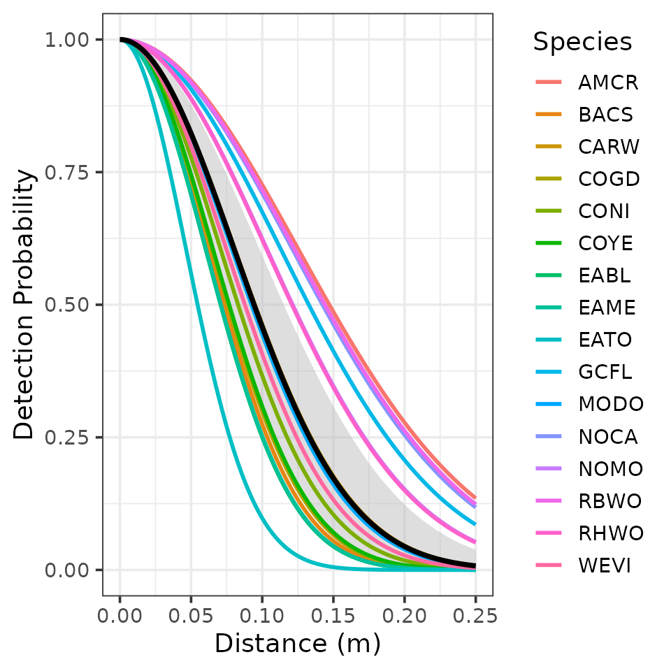
We see a fair amount of variation in detection probability across the species, with EATO having the quickest decay.
Posterior predictive checks
As with single-species models, we can use the ppcAbund()
function to perform posterior predictive checks, and summarize the check
with a Bayesian p-value using the summary() function. The
summary() function again requires the level
argument to specify if you want an overall Bayesian p-value for the
entire community (level = 'community'), each individual
species (level = 'species'), or for both
(level = 'both'). By default, we set `level = ‘both’.
ppc.ms.out <- ppcAbund(out.ms, fit.stat = 'chi-squared', group = 1)Currently on species 1 out of 16Currently on species 2 out of 16Currently on species 3 out of 16Currently on species 4 out of 16Currently on species 5 out of 16Currently on species 6 out of 16Currently on species 7 out of 16Currently on species 8 out of 16Currently on species 9 out of 16Currently on species 10 out of 16Currently on species 11 out of 16Currently on species 12 out of 16Currently on species 13 out of 16Currently on species 14 out of 16Currently on species 15 out of 16Currently on species 16 out of 16
summary(ppc.ms.out)
Call:
ppcAbund(object = out.ms, fit.stat = "chi-squared", group = 1)
Samples per Chain: 50000
Burn-in: 20000
Thinning Rate: 30
Number of Chains: 3
Total Posterior Samples: 3000
----------------------------------------
Community Level
----------------------------------------
Bayesian p-value: 0.4453
----------------------------------------
Species Level
----------------------------------------
EATO Bayesian p-value: 0.4373
EAME Bayesian p-value: 0.357
AMCR Bayesian p-value: 0.2367
BACS Bayesian p-value: 0.0497
CARW Bayesian p-value: 0.438
COGD Bayesian p-value: 0.361
CONI Bayesian p-value: 0.2093
COYE Bayesian p-value: 0.4993
EABL Bayesian p-value: 0.4587
GCFL Bayesian p-value: 0.6863
MODO Bayesian p-value: 0.445
NOCA Bayesian p-value: 0.3283
NOMO Bayesian p-value: 0.874
RBWO Bayesian p-value: 0.738
RHWO Bayesian p-value: 0.6853
WEVI Bayesian p-value: 0.3203
Fit statistic: chi-squared Model selection using WAIC
We can compute the WAIC for comparison with alternative models using
the waicAbund() function. For multi-species models, we can
calculate the WAIC for the entire data set, or we can calculate it
separately for each species. This is done by using the logical
by.sp argument. Note that the WAIC for the entire data set
is simply the sum of all the WAIC values for the individual responses.
Below we calculate the WAIC by species for the multi-species model and
compare the WAIC for species 1 to the corresponding WAIC for the
non-spatial single-species model we fit for that species.
# Multi-species HDS model
waicAbund(out.ms, by.sp = TRUE)N.max not specified. Setting upper index of integration of N to 10 plus
the largest estimated abundance value at each site in object$N.samplesCurrently on species 1 out of 16Currently on species 2 out of 16Currently on species 3 out of 16Currently on species 4 out of 16Currently on species 5 out of 16Currently on species 6 out of 16Currently on species 7 out of 16Currently on species 8 out of 16Currently on species 9 out of 16Currently on species 10 out of 16Currently on species 11 out of 16Currently on species 12 out of 16Currently on species 13 out of 16Currently on species 14 out of 16Currently on species 15 out of 16Currently on species 16 out of 16 elpd pD WAIC
1 -256.00212 4.969533 521.94331
2 -160.20401 4.352690 329.11340
3 -44.31214 4.043176 96.71064
4 -152.21178 6.975720 318.37500
5 -135.65333 4.383538 280.07374
6 -48.92443 3.681445 105.21175
7 -50.83144 4.526232 110.71535
8 -148.08196 4.335631 304.83518
9 -87.68360 3.018917 181.40504
10 -141.39292 3.807378 290.40059
11 -184.59930 4.131924 377.46244
12 -83.84912 3.461680 174.62160
13 -80.56650 2.569389 166.27177
14 -138.00114 3.061681 282.12565
15 -37.76504 3.171855 81.87380
16 -81.84562 4.766777 173.22479
# Single-species Poisson HDS model for EATO
waicAbund(out)N.max not specified. Setting upper index of integration of N to 10 plus
the largest estimated abundance value at each site in object$N.samples elpd pD WAIC
-255.728227 5.173769 521.803993 We could of course also run the same model with a negative binomial distribution for abundance, or using the negative exponential detection function.
Prediction
Prediction proceeds exactly as we have seen previously with the single-species non-spatial HDS model. Below we provide code to predict abundance and generate a map of total expected abundance across all species as a simple measure of “how many birds” we could expect at any given location (note the code is not run and can take a fair amount of memory).
# Recall what is in the prediction design matrix X.0
str(X.0)
out.ms.pred <- predict(out.ms, X.0)
# Note this takes a fair amount of memory to execute
str(out.ms.pred)
# Total expected abundance across all species at each site.
mu.sum.samples <- apply(out.ms.pred$mu.0.samples, c(1, 3), sum)
# Average total abundance at each site
mu.sum.means <- apply(mu.sum.samples, 2, mean)
plot.df <- data.frame(Easting = neonPredData$easting,
Northing = neonPredData$northing,
mu.sum.means = mu.sum.means)
coords.stars <- st_as_stars(plot.df, crs = st_crs(32617))
coords.sf <- st_as_sf(as.data.frame(neonDWP$coords), coords = c('easting', 'northing'),
crs = st_crs(32617))
# Plot of median estimate
ggplot() +
geom_stars(data = coords.stars, aes(x = Easting, y = Northing, fill = mu.sum.means)) +
geom_sf(data = coords.sf) +
scale_fill_viridis_c(na.value = NA) +
theme_bw(base_size = 14) +
labs(fill = 'Individuals\nper ha', x = 'Longitude', y = 'Latitude',
title = 'Average total density of birds')Latent factor multi-species HDS models
Basic model description
The latent factor multi-species HDS model is identical to the previously described multi-species HDS model except we include an additional component in the model to accommodate residual correlations between species. This type of model is often referred to as an abundance-based joint species distribution model (JSDM) in the statistical ecology literature (Warton et al. 2015). The previously described multi-species HDS model can be viewed as a simplified version of the latent factor multi-species HDS model, where we assume there are no residual correlations between species.
The model is identical to the previously described multi-species HDS model, with the only addition being a species-specific random effect at each site added to the equation for expected abundance. More specifically, we model species-specific abundance as
\[\begin{equation} \text{log}(\mu_{i, j}) = \boldsymbol{x}_j^\top\boldsymbol{\beta}_i + \text{w}^\ast_{i, j}. \end{equation}\]
The species-specific random effect \(\text{w}^\ast_{i, j}\) is used to account for residual correlations between species by assuming that correlation amongst the species can be explained by species-specific effects of a set of \(q\) latent variables. More specifically, we use a factor modeling approach (Lopes and West 2004) to account for species residual correlations in a computationally efficient manner (Tobler et al. 2019). This approach is ideal for large groups of species, where estimating a full \(I \times I\) covariance matrix would be computatinally intractable (and/or require massive amounts of data). Specifically, we decompose \(\text{w}^\ast_{i, j}\) into a linear combination of \(q\) latent variables (i.e., factors) and their associated species-specific coefficients (i.e., factor loadings) according to
\[\begin{equation}\label{factorModel} \text{w}^\ast_{i, j} = \boldsymbol{\lambda}_i^\top\text{w}_j, \end{equation}\]
where \(\boldsymbol{\lambda}_i^\top\) is the \(i\text{th}\) row of factor loadings from an \(I \times q\) loadings matrix \(\boldsymbol{\Lambda}\), and \(\text{w}_j\) is a \(q \times 1\) vector of independent latent factors at site \(j\). By settng \(q << N\), we achieve dimension reduction to efficiently model communities with a large number of species (Taylor-Rodriguez et al. 2019; Tobler et al. 2019; Doser, Finley, and Banerjee 2023). The approach accounts for residual species correlations via their species-specific responses to the \(q\) factors. We model each latent factor as a standard normal random variable. To ensure identifiability of the latent factors from the latent factor loadings, we fix the upper triangle of the factor loadings matrix to 0 and the diagonal elements to 1. We assign standard normal priors to the lower triangular elements of the factor loadings matrix. All other priors are identical to the multi-species HDS model previously discussed.
The constraints on the factor loadings matrix ensures identifiability
of the factor loadings from the latent factors, but this also results in
important practical considerations when fitting these models (e.g.,
ordering of the species, initial values). The spOccupancy
website provides a variety of vignettes that discuss these
considerations. All the advice applied to factor models fit with
detection-nondetection data in spOccupancy also apply to
factor models fit in spAbundance.
Fitting latent factor multi-species HDS models with
lfMsDS()
The function lfMsDS() fits latent factor multi-species
HDS models in spAbundance. The arguments are identical to
those in msDS() with one additional argument that specifies
the number of factors we wish to use in the model
(n.factors):
lfMsDS(abund.formula, det.formula, data, inits, priors,
tuning, n.factors, n.batch, batch.length, accept.rate = 0.43,
family = 'Poisson', transect = 'line', det.func = 'halfnormal',
n.omp.threads = 1, verbose = TRUE, n.report = 100,
n.burn = round(.10 * n.batch * batch.length), n.thin = 1,
n.chains = 1, ...)For guidance on choosing the number of latent factors, see the
section on fitting latent factor multi-species occupancy models on
the spOccupancy website. Here we will fit a model with a
single factor.
n.factors <- 1There are only a few slight differences in how we go about fitting a
multi-species HDS model with latent factors compared to one without
latent factors. The data format as well as
abund.formula and det.formula remain the same
as before.
List of 5
 $ y          : num [1:16, 1:90, 1:4] 0 0 0 0 0 0 1 0 0 0 ...
  ..- attr(*, "dimnames")=List of 3
  .. ..$ : chr [1:16] "EATO" "EAME" "AMCR" "BACS" ...
  .. ..$ : NULL
  .. ..$ : NULL
 $ covs       :'data.frame':    90 obs. of  4 variables:
  ..$ wind  : int [1:90] 0 0 0 1 0 0 1 0 0 1 ...
  ..$ day   : num [1:90] 132 132 132 132 132 132 132 132 132 129 ...
  ..$ forest: num [1:90] 0.18 0.0962 0.0577 0.1569 0.08 ...
  ..$ grass : num [1:90] 0.2 0.192 0.192 0.216 0.22 ...
 $ dist.breaks: num [1:5] 0 0.025 0.05 0.1 0.25
 $ offset     : num 19.6
 $ coords     : num [1:90, 1:2] 458629 458879 459129 458629 458879 ...
  ..- attr(*, "dimnames")=List of 2
  .. ..$ : NULL
.. ..$ : chr [1:2] "easting" "northing"Initial values are specified as with msDS(), with the
exception that we can now specify initial values for the latent factor
loadings matrix lambda and the latent factors
w. Initial values for the species-specific factor loadings
(lambda) are specified as a numeric matrix with \(I\) rows and \(q\) columns, where \(I\) is the number of species and \(q\) is the number of latent factors used in
the model. The diagonal elements of the matrix must be 1, and values in
the upper triangle must be set to 0 to ensure identifiability of the
latent factors. Note that the default initial values for the lower
triangle of the factor loadings matrix is 0. Below we set these default
values to random values from a standard normal distribution (the prior
distribution). We can also specify the initial values for the latent
factors. Below we set these to 0 (which is the default).
# Initiate all lambda initial values to 0.
lambda.inits <- matrix(0, n.sp, n.factors)
# Set diagonal elements to 1
diag(lambda.inits) <- 1
# Set lower triangular elements to random values from a standard normal distribution
lambda.inits[lower.tri(lambda.inits)] <- rnorm(sum(lower.tri(lambda.inits)))
# Make sure it's a matrix
lambda.inits <- as.matrix(lambda.inits)
# Check it out.
lambda.inits [,1]
[1,] 1.000000000
[2,] -0.023587171
[3,] -0.647174229
[4,] 1.116599778
[5,] 0.094833926
[6,] 1.773230720
[7,] 0.629039432
[8,] 0.623396492
[9,] -1.642673618
[10,] 0.908293438
[11,] -0.822336401
[12,] -0.352766710
[13,] -0.080026349
[14,] 0.001824156
[15,] 0.432969602
[16,] 0.704597196
w.inits <- matrix(0, n.factors, ncol(neonDWP$y))
ms.inits <- list(alpha.comm = 0,
beta.comm = 0,
beta = 0,
alpha = 0,
tau.sq.beta = 1,
kappa = 1,
tau.sq.alpha = 1,
sigma.sq.mu = 0.5,
lambda = lambda.inits,
w = w.inits,
N = apply(neonDWP$y, c(1, 2), sum, na.rm = TRUE))Priors are specified exactly the same as we saw with
msDS(). We do not need to explicitly specify the prior for
the factor loadings, as we require the prior for the lower-triangular
values to be Normal(0, 1).
ms.priors <- list(beta.comm.normal = list(mean = 0, var = 100),
alpha.comm.normal = list(mean = 0, var = 100),
tau.sq.beta.ig = list(a = 0.1, b = 0.1),
tau.sq.alpha.ig = list(a = 0.1, b = 0.1),
kappa.unif = list(a = 0, b = 100))We finish up by specifying the tuning values, where now we specify
the initial tuning variance for the factor loadings lambda
as well as the latent factors w. We then run the model for
a single chain of 50,000 iterations (2000 batches of length 25) with a
burn-in of 20,000 samples and a thinning rate of 30. For a complete
analysis we would run multiple chains, but here we use a single chain to
keep run times reasonable for example purposes. We will fit the model
with a Poisson distribution for abundance.
# Specify initial tuning values
ms.tuning <- list(beta = 0.3, alpha = 0.3, beta.star = 0.5, kappa = 0.5,
w = 0.5, lambda = 0.5)
# Approx. run time: 2.5 min
out.lf.ms <- lfMsDS(abund.formula = abund.formula,
det.formula = det.formula,
data = neonDWP,
inits = ms.inits,
n.batch = 2000,
tuning = ms.tuning,
batch.length = 25,
priors = ms.priors,
n.omp.threads = 1,
n.factors = n.factors,
family = 'Poisson',
det.func = 'halfnormal',
transect = 'point',
verbose = TRUE,
n.report = 500,
n.burn = 20000,
n.thin = 30,
n.chains = 1)----------------------------------------
Preparing to run the model
----------------------------------------
----------------------------------------
Model description
----------------------------------------
Latent Factor Multi-species Poisson HDS model with 90 sites and 16 species.
Samples per Chain: 50000 (2000 batches of length 25)
Burn-in: 20000
Thinning Rate: 30
Number of Chains: 1
Total Posterior Samples: 1000
Using 1 latent factors.
Source compiled with OpenMP support and model fit using 1 thread(s).
Adaptive Metropolis with target acceptance rate: 43.0
----------------------------------------
Chain 1
----------------------------------------
Sampling ...
Batch: 500 of 2000, 25.00%
Species Parameter Acceptance Tuning
1 beta[1] 36.0 0.05647
1 alpha[1] 40.0 0.07934
2 beta[1] 40.0 0.11837
2 alpha[1] 36.0 0.12822
3 beta[1] 56.0 0.47049
3 alpha[1] 52.0 0.33488
4 beta[1] 52.0 0.12320
4 alpha[1] 32.0 0.12822
5 beta[1] 44.0 0.15978
5 alpha[1] 48.0 0.12822
6 beta[1] 44.0 0.23836
6 alpha[1] 40.0 0.22448
7 beta[1] 48.0 0.31538
7 alpha[1] 44.0 0.30914
8 beta[1] 40.0 0.14171
8 alpha[1] 48.0 0.12822
9 beta[1] 40.0 0.15047
9 alpha[1] 52.0 0.16630
10 beta[1] 76.0 0.20312
10 alpha[1] 52.0 0.16966
11 beta[1] 32.0 0.12822
11 alpha[1] 44.0 0.10498
12 beta[1] 56.0 0.32175
12 alpha[1] 36.0 0.23836
13 beta[1] 52.0 0.23364
13 alpha[1] 64.0 0.18379
14 beta[1] 44.0 0.22003
14 alpha[1] 28.0 0.15661
15 beta[1] 40.0 0.39299
15 alpha[1] 32.0 0.29113
16 beta[1] 60.0 0.22003
16 alpha[1] 60.0 0.20722
-------------------------------------------------
Batch: 1000 of 2000, 50.00%
Species Parameter Acceptance Tuning
1 beta[1] 40.0 0.05997
1 alpha[1] 40.0 0.07472
2 beta[1] 32.0 0.11837
2 alpha[1] 32.0 0.12076
3 beta[1] 56.0 0.47049
3 alpha[1] 40.0 0.32175
4 beta[1] 48.0 0.11837
4 alpha[1] 44.0 0.12822
5 beta[1] 36.0 0.15978
5 alpha[1] 52.0 0.13615
6 beta[1] 56.0 0.28537
6 alpha[1] 40.0 0.25821
7 beta[1] 48.0 0.30914
7 alpha[1] 48.0 0.26343
8 beta[1] 48.0 0.12822
8 alpha[1] 48.0 0.13615
9 beta[1] 24.0 0.14457
9 alpha[1] 32.0 0.16630
10 beta[1] 48.0 0.21141
10 alpha[1] 56.0 0.15047
11 beta[1] 44.0 0.12822
11 alpha[1] 36.0 0.12320
12 beta[1] 48.0 0.32825
12 alpha[1] 40.0 0.22448
13 beta[1] 28.0 0.23836
13 alpha[1] 56.0 0.17658
14 beta[1] 28.0 0.20312
14 alpha[1] 40.0 0.15351
15 beta[1] 36.0 0.41729
15 alpha[1] 40.0 0.31538
16 beta[1] 44.0 0.20312
16 alpha[1] 40.0 0.17658
-------------------------------------------------
Batch: 1500 of 2000, 75.00%
Species Parameter Acceptance Tuning
1 beta[1] 44.0 0.05319
1 alpha[1] 52.0 0.07934
2 beta[1] 48.0 0.12320
2 alpha[1] 36.0 0.12076
3 beta[1] 52.0 0.43432
3 alpha[1] 60.0 0.34165
4 beta[1] 32.0 0.11372
4 alpha[1] 52.0 0.12569
5 beta[1] 44.0 0.16301
5 alpha[1] 48.0 0.13081
6 beta[1] 44.0 0.27418
6 alpha[1] 52.0 0.26343
7 beta[1] 48.0 0.32825
7 alpha[1] 52.0 0.28537
8 beta[1] 44.0 0.13890
8 alpha[1] 36.0 0.12822
9 beta[1] 44.0 0.15978
9 alpha[1] 44.0 0.18750
10 beta[1] 24.0 0.18015
10 alpha[1] 36.0 0.14749
11 beta[1] 48.0 0.13081
11 alpha[1] 56.0 0.11147
12 beta[1] 48.0 0.34855
12 alpha[1] 40.0 0.24318
13 beta[1] 36.0 0.21568
13 alpha[1] 52.0 0.16966
14 beta[1] 24.0 0.18750
14 alpha[1] 40.0 0.17308
15 beta[1] 48.0 0.38521
15 alpha[1] 56.0 0.28537
16 beta[1] 56.0 0.23364
16 alpha[1] 40.0 0.19515
-------------------------------------------------
Batch: 2000 of 2000, 100.00%
summary(out.lf.ms)
Call:
lfMsDS(abund.formula = abund.formula, det.formula = det.formula,
data = neonDWP, inits = ms.inits, priors = ms.priors, tuning = ms.tuning,
n.factors = n.factors, n.batch = 2000, batch.length = 25,
family = "Poisson", transect = "point", det.func = "halfnormal",
n.omp.threads = 1, verbose = TRUE, n.report = 500, n.burn = 20000,
n.thin = 30, n.chains = 1)
Samples per Chain: 50000
Burn-in: 20000
Thinning Rate: 30
Number of Chains: 1
Total Posterior Samples: 1000
Run Time (min): 2.1242
----------------------------------------
Community Level
----------------------------------------
Abundance Means (log scale):
Mean SD 2.5% 50% 97.5% Rhat ESS
(Intercept) -2.4883 0.3149 -3.1233 -2.4849 -1.8703 NA 389
scale(forest) -0.0630 0.0956 -0.2629 -0.0602 0.1175 NA 794
scale(grass) 0.0635 0.1209 -0.1767 0.0703 0.3136 NA 660
Abundance Variances (log scale):
Mean SD 2.5% 50% 97.5% Rhat ESS
(Intercept) 1.5411 0.6746 0.6873 1.3890 3.2306 NA 613
scale(forest) 0.1088 0.0608 0.0340 0.0954 0.2585 NA 476
scale(grass) 0.1834 0.0978 0.0650 0.1634 0.4381 NA 560
Detection Means (log scale):
Mean SD 2.5% 50% 97.5% Rhat ESS
(Intercept) -2.5313 0.1030 -2.7247 -2.5347 -2.3164 NA 605
scale(wind) -0.0161 0.0579 -0.1242 -0.0164 0.0991 NA 857
Detection Variances (log scale):
Mean SD 2.5% 50% 97.5% Rhat ESS
(Intercept) 0.1400 0.0736 0.0515 0.1241 0.3342 NA 563
scale(wind) 0.0378 0.0180 0.0157 0.0330 0.0838 NA 823
----------------------------------------
Species Level
----------------------------------------
Abundance (log scale):
Mean SD 2.5% 50% 97.5% Rhat ESS
(Intercept)-EATO -0.0822 0.1768 -0.4374 -0.0796 0.2387 NA 51
(Intercept)-EAME -1.4247 0.2208 -1.8890 -1.4116 -0.9974 NA 121
(Intercept)-AMCR -4.1458 0.4230 -4.9517 -4.1369 -3.3466 NA 259
(Intercept)-BACS -1.7245 0.2586 -2.2318 -1.7167 -1.2292 NA 85
(Intercept)-CARW -2.0766 0.2535 -2.5918 -2.0743 -1.5779 NA 161
(Intercept)-COGD -3.0355 0.4216 -3.8881 -3.0329 -2.2243 NA 100
(Intercept)-CONI -3.5597 0.4766 -4.5641 -3.5236 -2.7281 NA 120
(Intercept)-COYE -1.5934 0.2249 -2.0070 -1.5948 -1.1464 NA 132
(Intercept)-EABL -2.1055 0.3315 -2.7225 -2.1086 -1.4453 NA 103
(Intercept)-GCFL -2.4164 0.2547 -2.9405 -2.4097 -1.9114 NA 180
(Intercept)-MODO -1.5277 0.1921 -1.9047 -1.5317 -1.1590 NA 139
(Intercept)-NOCA -3.5883 0.3731 -4.3846 -3.5929 -2.8783 NA 171
(Intercept)-NOMO -3.3305 0.3469 -4.0638 -3.2988 -2.6570 NA 200
(Intercept)-RBWO -2.4615 0.2216 -2.8629 -2.4647 -2.0153 NA 220
(Intercept)-RHWO -4.1575 0.4893 -5.1468 -4.1405 -3.2504 NA 219
(Intercept)-WEVI -2.9528 0.3714 -3.7074 -2.9367 -2.2476 NA 136
scale(forest)-EATO 0.2087 0.1256 -0.0411 0.2104 0.4482 NA 128
scale(forest)-EAME 0.2204 0.1243 -0.0282 0.2192 0.4797 NA 320
scale(forest)-AMCR 0.0297 0.2110 -0.3944 0.0329 0.4399 NA 841
scale(forest)-BACS -0.0058 0.1504 -0.3024 -0.0076 0.3061 NA 272
scale(forest)-CARW -0.1114 0.1499 -0.4019 -0.1100 0.1784 NA 371
scale(forest)-COGD -0.3417 0.2305 -0.8059 -0.3333 0.0825 NA 355
scale(forest)-CONI -0.1719 0.2225 -0.5766 -0.1623 0.2761 NA 528
scale(forest)-COYE 0.0612 0.1316 -0.1923 0.0579 0.3209 NA 387
scale(forest)-EABL -0.0765 0.1718 -0.4226 -0.0844 0.2623 NA 335
scale(forest)-GCFL -0.0075 0.1348 -0.2569 -0.0085 0.2525 NA 621
scale(forest)-MODO -0.2298 0.1114 -0.4400 -0.2294 -0.0202 NA 338
scale(forest)-NOCA 0.0074 0.1857 -0.3594 0.0025 0.3851 NA 513
scale(forest)-NOMO 0.2395 0.1631 -0.0651 0.2348 0.5748 NA 416
scale(forest)-RBWO -0.1638 0.1243 -0.4040 -0.1624 0.0648 NA 838
scale(forest)-RHWO -0.6788 0.2773 -1.2502 -0.6569 -0.1916 NA 392
scale(forest)-WEVI 0.0473 0.2112 -0.3493 0.0547 0.4706 NA 397
scale(grass)-EATO -0.0199 0.1353 -0.2939 -0.0105 0.2183 NA 86
scale(grass)-EAME 0.3430 0.1356 0.0935 0.3377 0.6215 NA 260
scale(grass)-AMCR -0.1656 0.2487 -0.6724 -0.1620 0.3113 NA 768
scale(grass)-BACS -0.0573 0.1722 -0.4094 -0.0576 0.2766 NA 199
scale(grass)-CARW -0.1208 0.1677 -0.4710 -0.1130 0.1867 NA 223
scale(grass)-COGD 0.0354 0.2505 -0.4410 0.0455 0.5120 NA 293
scale(grass)-CONI 0.1745 0.2582 -0.3446 0.1865 0.6553 NA 438
scale(grass)-COYE -0.1335 0.1375 -0.4007 -0.1361 0.1286 NA 340
scale(grass)-EABL -0.0855 0.1844 -0.4721 -0.0778 0.2414 NA 335
scale(grass)-GCFL -0.1020 0.1382 -0.3803 -0.0996 0.1805 NA 451
scale(grass)-MODO 0.1936 0.1140 -0.0260 0.1926 0.4241 NA 471
scale(grass)-NOCA 0.0253 0.2174 -0.4257 0.0244 0.4514 NA 253
scale(grass)-NOMO 1.1991 0.2405 0.7362 1.1983 1.6810 NA 430
scale(grass)-RBWO -0.1187 0.1304 -0.3702 -0.1198 0.1393 NA 702
scale(grass)-RHWO -0.1500 0.2622 -0.6546 -0.1481 0.3760 NA 653
scale(grass)-WEVI -0.0834 0.2113 -0.5160 -0.0827 0.2976 NA 303
Detection (log scale):
Mean SD 2.5% 50% 97.5% Rhat ESS
(Intercept)-EATO -3.0719 0.0445 -3.1578 -3.0718 -2.9852 NA 119
(Intercept)-EAME -2.7941 0.0713 -2.9317 -2.7978 -2.6436 NA 224
(Intercept)-AMCR -2.1047 0.2532 -2.5017 -2.1398 -1.5404 NA 313
(Intercept)-BACS -2.7854 0.0780 -2.9286 -2.7885 -2.6313 NA 245
(Intercept)-CARW -2.5283 0.0996 -2.7068 -2.5330 -2.3113 NA 171
(Intercept)-COGD -2.7584 0.1538 -3.0544 -2.7625 -2.4313 NA 161
(Intercept)-CONI -2.6615 0.1782 -2.9877 -2.6655 -2.2635 NA 246
(Intercept)-COYE -2.7243 0.0845 -2.8938 -2.7266 -2.5613 NA 173
(Intercept)-EABL -2.8277 0.1082 -3.0361 -2.8303 -2.6060 NA 111
(Intercept)-GCFL -2.2332 0.1343 -2.4543 -2.2498 -1.9273 NA 215
(Intercept)-MODO -2.5448 0.0732 -2.6785 -2.5467 -2.3989 NA 230
(Intercept)-NOCA -2.1360 0.2036 -2.4476 -2.1643 -1.6872 NA 239
(Intercept)-NOMO -2.3081 0.1357 -2.5502 -2.3174 -2.0090 NA 264
(Intercept)-RBWO -2.1181 0.1423 -2.3557 -2.1316 -1.8007 NA 213
(Intercept)-RHWO -2.3079 0.2402 -2.7278 -2.3228 -1.8099 NA 282
(Intercept)-WEVI -2.6088 0.1269 -2.8344 -2.6105 -2.3452 NA 265
scale(wind)-EATO -0.0653 0.0383 -0.1408 -0.0655 0.0166 NA 359
scale(wind)-EAME 0.0348 0.0428 -0.0540 0.0351 0.1163 NA 605
scale(wind)-AMCR -0.0074 0.1311 -0.2533 -0.0127 0.2761 NA 797
scale(wind)-BACS -0.2327 0.0835 -0.4080 -0.2287 -0.0811 NA 477
scale(wind)-CARW 0.0079 0.0751 -0.1291 0.0062 0.1615 NA 710
scale(wind)-COGD 0.0894 0.0922 -0.0802 0.0859 0.2782 NA 1000
scale(wind)-CONI -0.0060 0.0971 -0.1823 -0.0111 0.1913 NA 772
scale(wind)-COYE -0.0639 0.0700 -0.1998 -0.0617 0.0726 NA 653
scale(wind)-EABL -0.0264 0.0806 -0.1792 -0.0287 0.1443 NA 824
scale(wind)-GCFL -0.0086 0.0706 -0.1442 -0.0084 0.1301 NA 696
scale(wind)-MODO -0.0623 0.0500 -0.1575 -0.0629 0.0394 NA 950
scale(wind)-NOCA -0.0576 0.1230 -0.2966 -0.0594 0.1850 NA 744
scale(wind)-NOMO 0.2456 0.0968 0.0880 0.2376 0.4633 NA 383
scale(wind)-RBWO 0.0688 0.0818 -0.0772 0.0663 0.2502 NA 499
scale(wind)-RHWO -0.1917 0.1634 -0.5202 -0.1899 0.1413 NA 814
scale(wind)-WEVI -0.0003 0.0926 -0.1817 -0.0001 0.1792 NA 587Note that the factor loadings themselves are not shown in the
summary() output, but are available in the
lambda.samples portion of the model list object.
# ESS for lambda
out.lf.ms$ESS$lambda EATO-1 EAME-1 AMCR-1 BACS-1 CARW-1 COGD-1 CONI-1 COYE-1
0.00000 99.22126 206.27811 38.38516 195.84434 129.22036 64.60092 152.91945
EABL-1 GCFL-1 MODO-1 NOCA-1 NOMO-1 RBWO-1 RHWO-1 WEVI-1
164.70237 355.35448 126.48185 176.80013 167.06664 378.14479 229.58785 153.16638
# Posterior quantiles for the latent factor loadings
summary(out.lf.ms$lambda.samples)$quantiles 2.5% 25% 50% 75% 97.5%
EATO-1 1.00000000 1.00000000 1.0000000 1.00000000 1.00000000
EAME-1 -0.97740605 -0.61658624 -0.4696155 -0.30619549 -0.01558045
AMCR-1 -0.81387785 -0.19051220 0.1201048 0.45189102 1.15273177
BACS-1 -1.74599434 -1.38562569 -1.1499378 -0.89942683 -0.40592449
CARW-1 0.06268297 0.43687061 0.6364128 0.81808401 1.22226318
COGD-1 -0.71875887 -0.11266040 0.2300554 0.57689206 1.24906043
CONI-1 -2.05915233 -1.30648498 -0.8892407 -0.50647936 0.44616703
COYE-1 -0.59248942 -0.26620074 -0.1063640 0.07141423 0.39590305
EABL-1 -1.08742598 -0.67090086 -0.4335337 -0.20214031 0.29613607
GCFL-1 0.06785623 0.30574890 0.4622588 0.62516419 0.92730519
MODO-1 -0.16910329 0.11133259 0.2557478 0.40350848 0.74987570
NOCA-1 0.35777486 0.83873414 1.0811640 1.36177157 1.86506720
NOMO-1 -0.32788248 -0.02895023 0.1730366 0.37370216 0.77385097
RBWO-1 -0.31366629 -0.02812946 0.1154850 0.26238722 0.53870444
RHWO-1 -0.69386285 -0.04904413 0.2811197 0.63695552 1.33405250
WEVI-1 0.36507576 0.86303891 1.1234650 1.42200239 2.06456547We can inspect the latent factor loadings as well as the latent
factors (stored in out.lf.ms$w.samples) to provide
information on any groupings that arise from the species in the modeled
community. See Appendix S1 in Doser, Finley, and
Banerjee (2023) for a discussion on using factor models as a
model-based ordination technique.
Posterior predictive checks
We again use the ppcAbund() function perform a posterior
predictive check of our model
ppc.out.lf.ms <- ppcAbund(out.lf.ms, fit.stat = 'chi-squared', group = 1)Currently on species 1 out of 16Currently on species 2 out of 16Currently on species 3 out of 16Currently on species 4 out of 16Currently on species 5 out of 16Currently on species 6 out of 16Currently on species 7 out of 16Currently on species 8 out of 16Currently on species 9 out of 16Currently on species 10 out of 16Currently on species 11 out of 16Currently on species 12 out of 16Currently on species 13 out of 16Currently on species 14 out of 16Currently on species 15 out of 16Currently on species 16 out of 16
# Summarize with a Bayesian p-value
summary(ppc.out.lf.ms)
Call:
ppcAbund(object = out.lf.ms, fit.stat = "chi-squared", group = 1)
Samples per Chain: 50000
Burn-in: 20000
Thinning Rate: 30
Number of Chains: 1
Total Posterior Samples: 1000
----------------------------------------
Community Level
----------------------------------------
Bayesian p-value: 0.4728
----------------------------------------
Species Level
----------------------------------------
EATO Bayesian p-value: 0.153
EAME Bayesian p-value: 0.352
AMCR Bayesian p-value: 0.227
BACS Bayesian p-value: 0.229
CARW Bayesian p-value: 0.496
COGD Bayesian p-value: 0.324
CONI Bayesian p-value: 0.378
COYE Bayesian p-value: 0.467
EABL Bayesian p-value: 0.438
GCFL Bayesian p-value: 0.763
MODO Bayesian p-value: 0.492
NOCA Bayesian p-value: 0.513
NOMO Bayesian p-value: 0.881
RBWO Bayesian p-value: 0.687
RHWO Bayesian p-value: 0.656
WEVI Bayesian p-value: 0.508
Fit statistic: chi-squared Model selection using WAIC
We can use waicAbund() to calculate the WAIC for
comparison to other models. Below, we compare the regular multi-species
HDS model to the latent factor multi-species HDS model.
# With latent factors
waicAbund(out.lf.ms, by.sp = TRUE)N.max not specified. Setting upper index of integration of N to 10 plus
the largest estimated abundance value at each site in object$N.samplesCurrently on species 1 out of 16Currently on species 2 out of 16Currently on species 3 out of 16Currently on species 4 out of 16Currently on species 5 out of 16Currently on species 6 out of 16Currently on species 7 out of 16Currently on species 8 out of 16Currently on species 9 out of 16Currently on species 10 out of 16Currently on species 11 out of 16Currently on species 12 out of 16Currently on species 13 out of 16Currently on species 14 out of 16Currently on species 15 out of 16Currently on species 16 out of 16 elpd pD WAIC
1 -251.41364 32.232430 567.29214
2 -154.92031 8.240509 326.32165
3 -43.42008 5.617762 98.07569
4 -126.15607 24.205398 300.72294
5 -129.42362 8.948662 276.74456
6 -48.06946 5.282682 106.70429
7 -44.94058 10.399852 110.68087
8 -147.46988 5.892217 306.72419
9 -85.37152 5.226845 181.19673
10 -137.73898 5.775653 287.02926
11 -182.06488 6.790577 377.71091
12 -73.63756 8.869001 165.01312
13 -80.06064 3.522127 167.16553
14 -137.66758 3.973684 283.28254
15 -36.66088 4.481308 82.28438
16 -72.48177 9.716312 164.39616
# Without latent factors
waicAbund(out.ms, by.sp = TRUE)N.max not specified. Setting upper index of integration of N to 10 plus
the largest estimated abundance value at each site in object$N.samplesCurrently on species 1 out of 16Currently on species 2 out of 16Currently on species 3 out of 16Currently on species 4 out of 16Currently on species 5 out of 16Currently on species 6 out of 16Currently on species 7 out of 16Currently on species 8 out of 16Currently on species 9 out of 16Currently on species 10 out of 16Currently on species 11 out of 16Currently on species 12 out of 16Currently on species 13 out of 16Currently on species 14 out of 16Currently on species 15 out of 16Currently on species 16 out of 16 elpd pD WAIC
1 -256.00212 4.969533 521.94331
2 -160.20401 4.352690 329.11340
3 -44.31214 4.043176 96.71064
4 -152.21178 6.975720 318.37500
5 -135.65333 4.383538 280.07374
6 -48.92443 3.681445 105.21175
7 -50.83144 4.526232 110.71535
8 -148.08196 4.335631 304.83518
9 -87.68360 3.018917 181.40504
10 -141.39292 3.807378 290.40059
11 -184.59930 4.131924 377.46244
12 -83.84912 3.461680 174.62160
13 -80.56650 2.569389 166.27177
14 -138.00114 3.061681 282.12565
15 -37.76504 3.171855 81.87380
16 -81.84562 4.766777 173.22479We see that accommodating species correlations appears to improve model fit for some species, but not for others.
Prediction
Prediction proceeds exactly as before with the multi-species HDS model, with the only exception being that we need to provide the spatial coordinates for prediction. This is because if predicting at sites where the data were observed, using the latent factors in the prediction can provide substantial improvements.
# Note this takes a fair amount of memory to execute (not run)
out.lf.ms.pred <- predict(out.lf.ms, X.0, coords.0)Spatial factor multi-species HDS models
Basic model description
Our final model is a spatially-explicit extension of the latent factor multi-species HDS model, where we now account for species correlations and spatial autocorrelation. We do this using a spatial factor modeling approach (Hogan and Tchernis 2004), which is almost identical to the previous latent factor model, but now instead of modeling the latent factors \(\textbf{w}\) as standard normal random variables, we model them as spatial factors. More specifically, we model each of the spatial factors using an independent NNGP, which is identical to how we modeled spatial autocorrelation for a single species with the only exception being that we fix the spatial variance parameter \(\sigma^2\) to 1 to ensure identifiability (Taylor-Rodriguez et al. 2019). We estimate all the parameters we estimated for the latent factor multi-species HDS model, with the addition of \(q\) spatial decay parameters (one for each of the estimated spatial factors), which we model with a uniform prior as we did in the single-species spatial HDS model. This model can be viewed as an abundance-based JSDM that simultaneously accounts for imperfect detection, spatial autocorrelation, and species correlations. Compared to the latent factor multi-species HDS model, the spatial factor model will likely provide improved predictive performance, as the spatial structure of the latent factors allows us to share information across space, including non-sampled locations. For more details on a similar model in the context of occupancy models, see Doser, Finley, and Banerjee (2023).
Fitting spatial factor multi-species HDS models with
sfMsDS()
The function sfMsDS() fits spatial factor multi-species
HDS models.
sfMsDS(abund.formula, det.formula, data, inits, priors,
tuning, cov.model = 'exponential', NNGP = TRUE,
n.neighbors = 15, search.type = 'cb', n.factors,
n.batch, batch.length, accept.rate = 0.43,
family = 'Poisson', transect = 'line', det.func = 'halfnormal',
n.omp.threads = 1, verbose = TRUE, n.report = 100,
n.burn = round(.10 * n.batch * batch.length), n.thin = 1,
n.chains = 1, ...)We have already discussed all the components required for fitting
models with sfMsDS() as it has the same arguments as
lfMSDS() as well as the additional arguments for fitting
spatial models that we saw with spDS(). Below we run all
the code for fitting the same model as we did with
lfMsDS(), but now accommodating spatial autocorrelation in
the latent factors. Notice the main difference in preparing the model
arguments for fitting a model with sfMsDS() compared to
lfMsDS() is the addition of the spatial decay parameters
phi in the initial values, priors, and tuning variances.
Note that out of all the models discussed, sfMsDS() is the
slowest model (which makes sense since it is also the most
complicated).
# Formulas
abund.formula <- ~ scale(forest) + scale(grass)
det.formula <- ~ scale(wind)
# Initiate all lambda initial values to 0.
lambda.inits <- matrix(0, n.sp, n.factors)
# Set diagonal elements to 1
diag(lambda.inits) <- 1
# Set lower triangular elements to random values from a standard normal distribution
lambda.inits[lower.tri(lambda.inits)] <- rnorm(sum(lower.tri(lambda.inits)))
# Make sure it's a matrix
lambda.inits <- as.matrix(lambda.inits)
# Check it out.
lambda.inits
[,1]
[1,] 1.0000000
[2,] 0.4020850
[3,] -0.3534404
[4,] 1.0973512
[5,] 0.8597650
[6,] -0.3231153
[7,] -0.5126134
[8,] -0.6557710
[9,] -0.1908273
[10,] 1.3465453
[11,] -0.7127088
[12,] 1.4548454
[13,] 1.0233795
[14,] 1.2850208
[15,] -1.2018156
[16,] 0.6504345
# Pair-wise distances between all sites for initial values and prior for phi
dist.mat <- dist(neonDWP$coords)
w.inits <- matrix(0, n.factors, ncol(neonDWP$y))
ms.inits <- list(alpha.comm = 0,
beta.comm = 0,
beta = 0,
alpha = 0,
tau.sq.beta = 1,
kappa = 1,
phi = 3 / mean(dist.mat),
tau.sq.alpha = 1,
sigma.sq.mu = 0.5,
lambda = lambda.inits,
w = w.inits,
N = apply(neonDWP$y, c(1, 2), sum, na.rm = TRUE))
# Exponential covariance model
cov.model <- 'exponential'
# Priors
ms.priors <- list(beta.comm.normal = list(mean = 0, var = 100),
alpha.comm.normal = list(mean = 0, var = 100),
tau.sq.beta.ig = list(a = 0.1, b = 0.1),
tau.sq.alpha.ig = list(a = 0.1, b = 0.1),
phi.unif = list(a = 3 / max(dist.mat), 3 / min(dist.mat)),
kappa.unif = list(a = 0, b = 100))
# Specify initial tuning values
ms.tuning <- list(beta = 0.3, alpha = 0.3, beta.star = 0.5, kappa = 0.5,
w = 0.5, lambda = 0.5, phi = 0.5)
# Approx. run time: 2.88 min
out.sf.ms <- sfMsDS(abund.formula = abund.formula,
det.formula = det.formula,
data = neonDWP,
inits = ms.inits,
n.batch = 2000,
tuning = ms.tuning,
batch.length = 25,
priors = ms.priors,
n.omp.threads = 1,
n.factors = n.factors,
family = 'Poisson',
det.func = 'halfnormal',
cov.model = 'exponential',
NNGP = TRUE,
n.neighbors = 15,
transect = 'point',
verbose = TRUE,
n.report = 500,
n.burn = 20000,
n.thin = 30,
n.chains = 1)----------------------------------------
Preparing to run the model
----------------------------------------
----------------------------------------
Building the neighbor list
----------------------------------------
----------------------------------------
Building the neighbors of neighbors list
----------------------------------------
----------------------------------------
Model description
----------------------------------------
Spatial Factor Multi-species Poisson HDS model with 90 sites and 16 species.
Samples per Chain: 50000 (2000 batches of length 25)
Burn-in: 20000
Thinning Rate: 30
Number of Chains: 1
Total Posterior Samples: 1000
Using the exponential spatial correlation model.
Using 1 latent spatial factors.
Using 15 nearest neighbors.
Source compiled with OpenMP support and model fit using 1 thread(s).
Adaptive Metropolis with target acceptance rate: 43.0
----------------------------------------
Chain 1
----------------------------------------
Sampling ...
Batch: 500 of 2000, 25.00%
Number Parameter Acceptance Tuning
1 beta[1] 36.0 0.05536
1 alpha[1] 56.0 0.07934
2 beta[1] 28.0 0.12320
2 alpha[1] 40.0 0.11837
3 beta[1] 40.0 0.47049
3 alpha[1] 20.0 0.36277
4 beta[1] 32.0 0.13081
4 alpha[1] 40.0 0.12822
5 beta[1] 48.0 0.15978
5 alpha[1] 28.0 0.14457
6 beta[1] 44.0 0.27418
6 alpha[1] 52.0 0.25821
7 beta[1] 64.0 0.27418
7 alpha[1] 44.0 0.25821
8 beta[1] 28.0 0.13081
8 alpha[1] 28.0 0.12569
9 beta[1] 44.0 0.17658
9 alpha[1] 40.0 0.18015
10 beta[1] 28.0 0.19515
10 alpha[1] 44.0 0.13346
11 beta[1] 44.0 0.12822
11 alpha[1] 56.0 0.11602
12 beta[1] 40.0 0.26875
12 alpha[1] 44.0 0.20722
13 beta[1] 24.0 0.22448
13 alpha[1] 40.0 0.17658
14 beta[1] 36.0 0.20722
14 alpha[1] 56.0 0.15047
15 beta[1] 36.0 0.44309
15 alpha[1] 40.0 0.29113
16 beta[1] 44.0 0.21568
16 alpha[1] 52.0 0.19515
1 phi 28.0 2.35574
-------------------------------------------------
Batch: 1000 of 2000, 50.00%
Number Parameter Acceptance Tuning
1 beta[1] 48.0 0.05997
1 alpha[1] 44.0 0.07777
2 beta[1] 24.0 0.10086
2 alpha[1] 60.0 0.10710
3 beta[1] 20.0 0.41729
3 alpha[1] 28.0 0.32825
4 beta[1] 44.0 0.11602
4 alpha[1] 48.0 0.11602
5 beta[1] 48.0 0.15661
5 alpha[1] 36.0 0.13081
6 beta[1] 48.0 0.25821
6 alpha[1] 36.0 0.27972
7 beta[1] 60.0 0.29113
7 alpha[1] 60.0 0.27972
8 beta[1] 32.0 0.12569
8 alpha[1] 48.0 0.13615
9 beta[1] 48.0 0.16301
9 alpha[1] 36.0 0.17658
10 beta[1] 44.0 0.20722
10 alpha[1] 24.0 0.15047
11 beta[1] 40.0 0.12822
11 alpha[1] 40.0 0.11372
12 beta[1] 52.0 0.32825
12 alpha[1] 28.0 0.22901
13 beta[1] 36.0 0.24318
13 alpha[1] 48.0 0.17658
14 beta[1] 32.0 0.19129
14 alpha[1] 32.0 0.15047
15 beta[1] 56.0 0.36277
15 alpha[1] 20.0 0.30302
16 beta[1] 48.0 0.22448
16 alpha[1] 52.0 0.21568
1 phi 28.0 2.35574
-------------------------------------------------
Batch: 1500 of 2000, 75.00%
Number Parameter Acceptance Tuning
1 beta[1] 56.0 0.05536
1 alpha[1] 36.0 0.07324
2 beta[1] 36.0 0.10498
2 alpha[1] 56.0 0.11602
3 beta[1] 28.0 0.40903
3 alpha[1] 36.0 0.33488
4 beta[1] 36.0 0.13346
4 alpha[1] 28.0 0.12569
5 beta[1] 36.0 0.15978
5 alpha[1] 52.0 0.13346
6 beta[1] 48.0 0.22448
6 alpha[1] 36.0 0.24318
7 beta[1] 48.0 0.25310
7 alpha[1] 52.0 0.27972
8 beta[1] 52.0 0.12320
8 alpha[1] 40.0 0.12320
9 beta[1] 48.0 0.16966
9 alpha[1] 64.0 0.18015
10 beta[1] 36.0 0.20312
10 alpha[1] 48.0 0.16301
11 beta[1] 44.0 0.12822
11 alpha[1] 56.0 0.10927
12 beta[1] 28.0 0.31538
12 alpha[1] 40.0 0.23364
13 beta[1] 24.0 0.22448
13 alpha[1] 36.0 0.18015
14 beta[1] 52.0 0.20722
14 alpha[1] 64.0 0.15978
15 beta[1] 28.0 0.41729
15 alpha[1] 64.0 0.29113
16 beta[1] 32.0 0.22901
16 alpha[1] 44.0 0.19910
1 phi 48.0 2.55194
-------------------------------------------------
Batch: 2000 of 2000, 100.00%
summary(out.sf.ms)
Call:
sfMsDS(abund.formula = abund.formula, det.formula = det.formula,
data = neonDWP, inits = ms.inits, priors = ms.priors, tuning = ms.tuning,
cov.model = "exponential", NNGP = TRUE, n.neighbors = 15,
n.factors = n.factors, n.batch = 2000, batch.length = 25,
family = "Poisson", transect = "point", det.func = "halfnormal",
n.omp.threads = 1, verbose = TRUE, n.report = 500, n.burn = 20000,
n.thin = 30, n.chains = 1)
Samples per Chain: 50000
Burn-in: 20000
Thinning Rate: 30
Number of Chains: 1
Total Posterior Samples: 1000
Run Time (min): 2.8086
----------------------------------------
Community Level
----------------------------------------
Abundance Means (log scale):
Mean SD 2.5% 50% 97.5% Rhat ESS
(Intercept) -2.5808 0.3174 -3.2207 -2.5782 -1.9548 NA 768
scale(forest) -0.0514 0.0987 -0.2527 -0.0485 0.1408 NA 647
scale(grass) 0.0601 0.1212 -0.1819 0.0564 0.2997 NA 555
Abundance Variances (log scale):
Mean SD 2.5% 50% 97.5% Rhat ESS
(Intercept) 1.5440 0.7199 0.6634 1.3969 3.1170 NA 743
scale(forest) 0.1116 0.0730 0.0333 0.0965 0.2956 NA 509
scale(grass) 0.1992 0.1076 0.0666 0.1768 0.4702 NA 547
Detection Means (log scale):
Mean SD 2.5% 50% 97.5% Rhat ESS
(Intercept) -2.5295 0.1016 -2.7325 -2.5267 -2.3255 NA 595
scale(wind) -0.0178 0.0516 -0.1321 -0.0181 0.0813 NA 1000
Detection Variances (log scale):
Mean SD 2.5% 50% 97.5% Rhat ESS
(Intercept) 0.1425 0.0706 0.0583 0.1237 0.3260 NA 496
scale(wind) 0.0340 0.0170 0.0136 0.0305 0.0716 NA 904
----------------------------------------
Species Level
----------------------------------------
Abundance (log scale):
Mean SD 2.5% 50% 97.5% Rhat ESS
(Intercept)-EATO -0.1546 0.2415 -0.6542 -0.1672 0.3072 NA 18
(Intercept)-EAME -1.3604 0.2379 -1.8466 -1.3456 -0.9223 NA 102
(Intercept)-AMCR -4.0525 0.4250 -4.8863 -4.0590 -3.2225 NA 254
(Intercept)-BACS -2.4964 0.5391 -3.5353 -2.5039 -1.4375 NA 27
(Intercept)-CARW -1.9153 0.3186 -2.6120 -1.8999 -1.3107 NA 39
(Intercept)-COGD -3.0500 0.4199 -3.9528 -3.0336 -2.2538 NA 124
(Intercept)-CONI -3.9311 0.5754 -5.1419 -3.8787 -2.9663 NA 111
(Intercept)-COYE -1.7178 0.2499 -2.2309 -1.7038 -1.2817 NA 101
(Intercept)-EABL -2.3633 0.3694 -3.1448 -2.3597 -1.7086 NA 90
(Intercept)-GCFL -2.3700 0.2715 -2.9334 -2.3577 -1.8834 NA 101
(Intercept)-MODO -1.5548 0.2000 -1.9483 -1.5434 -1.1824 NA 165
(Intercept)-NOCA -3.2619 0.3955 -4.0330 -3.2549 -2.4441 NA 126
(Intercept)-NOMO -3.4572 0.4174 -4.3155 -3.4262 -2.7024 NA 136
(Intercept)-RBWO -2.4497 0.2391 -2.8964 -2.4531 -1.9873 NA 225
(Intercept)-RHWO -4.2226 0.4960 -5.2637 -4.1740 -3.3004 NA 223
(Intercept)-WEVI -2.7760 0.4616 -3.7079 -2.7549 -1.9194 NA 60
scale(forest)-EATO 0.1896 0.1018 -0.0054 0.1916 0.3957 NA 117
scale(forest)-EAME 0.2330 0.1237 0.0051 0.2299 0.4829 NA 252
scale(forest)-AMCR 0.0493 0.2276 -0.3958 0.0463 0.4860 NA 1033
scale(forest)-BACS -0.0240 0.1936 -0.3911 -0.0314 0.3735 NA 113
scale(forest)-CARW -0.1200 0.1478 -0.4094 -0.1192 0.1620 NA 417
scale(forest)-COGD -0.3197 0.2275 -0.7801 -0.3122 0.1180 NA 330
scale(forest)-CONI -0.1129 0.2132 -0.5714 -0.1059 0.2808 NA 429
scale(forest)-COYE 0.0484 0.1279 -0.1912 0.0490 0.2956 NA 308
scale(forest)-EABL -0.0583 0.1643 -0.3884 -0.0566 0.2609 NA 263
scale(forest)-GCFL -0.0025 0.1369 -0.2678 0.0029 0.2550 NA 682
scale(forest)-MODO -0.2045 0.1064 -0.4119 -0.2008 -0.0001 NA 474
scale(forest)-NOCA 0.0243 0.1824 -0.3299 0.0246 0.3957 NA 702
scale(forest)-NOMO 0.2857 0.1888 -0.0859 0.2751 0.6667 NA 596
scale(forest)-RBWO -0.1655 0.1292 -0.4098 -0.1609 0.0831 NA 756
scale(forest)-RHWO -0.6537 0.3002 -1.3105 -0.6196 -0.1003 NA 392
scale(forest)-WEVI 0.0471 0.2245 -0.4047 0.0550 0.4806 NA 418
scale(grass)-EATO 0.0578 0.1211 -0.1815 0.0567 0.2919 NA 97
scale(grass)-EAME 0.3293 0.1412 0.0634 0.3200 0.6181 NA 260
scale(grass)-AMCR -0.1523 0.2335 -0.6134 -0.1488 0.3148 NA 841
scale(grass)-BACS 0.0154 0.2330 -0.4342 0.0096 0.4953 NA 127
scale(grass)-CARW -0.2192 0.1676 -0.5459 -0.2158 0.1186 NA 277
scale(grass)-COGD 0.0465 0.2447 -0.4291 0.0399 0.5264 NA 372
scale(grass)-CONI 0.2772 0.2864 -0.2728 0.2738 0.8331 NA 337
scale(grass)-COYE -0.0996 0.1550 -0.4126 -0.0999 0.2028 NA 246
scale(grass)-EABL -0.0164 0.1992 -0.4015 -0.0198 0.3641 NA 248
scale(grass)-GCFL -0.1387 0.1354 -0.3924 -0.1415 0.1241 NA 446
scale(grass)-MODO 0.1982 0.1207 -0.0339 0.1951 0.4306 NA 472
scale(grass)-NOCA -0.0470 0.1962 -0.4403 -0.0482 0.3125 NA 367
scale(grass)-NOMO 1.2006 0.2533 0.7053 1.2114 1.6753 NA 242
scale(grass)-RBWO -0.1430 0.1309 -0.3984 -0.1418 0.1189 NA 612
scale(grass)-RHWO -0.1636 0.2624 -0.6800 -0.1721 0.3517 NA 639
scale(grass)-WEVI -0.1826 0.2255 -0.6300 -0.1731 0.2424 NA 163
Detection (log scale):
Mean SD 2.5% 50% 97.5% Rhat ESS
(Intercept)-EATO -3.0735 0.0440 -3.1547 -3.0748 -2.9871 NA 196
(Intercept)-EAME -2.8126 0.0710 -2.9412 -2.8146 -2.6739 NA 176
(Intercept)-AMCR -2.1241 0.2475 -2.5106 -2.1612 -1.5405 NA 292
(Intercept)-BACS -2.7598 0.0805 -2.9183 -2.7585 -2.6004 NA 268
(Intercept)-CARW -2.5374 0.0934 -2.7119 -2.5399 -2.3398 NA 243
(Intercept)-COGD -2.7504 0.1531 -3.0250 -2.7550 -2.4356 NA 179
(Intercept)-CONI -2.6880 0.1751 -3.0070 -2.6947 -2.3248 NA 180
(Intercept)-COYE -2.7319 0.0814 -2.8865 -2.7341 -2.5611 NA 211
(Intercept)-EABL -2.8161 0.1030 -3.0007 -2.8184 -2.6142 NA 256
(Intercept)-GCFL -2.2070 0.1437 -2.4360 -2.2258 -1.8773 NA 140
(Intercept)-MODO -2.5372 0.0738 -2.6703 -2.5402 -2.3873 NA 263
(Intercept)-NOCA -2.1290 0.2098 -2.4668 -2.1544 -1.6829 NA 220
(Intercept)-NOMO -2.2674 0.1515 -2.5269 -2.2805 -1.9221 NA 249
(Intercept)-RBWO -2.1025 0.1540 -2.3500 -2.1129 -1.8002 NA 176
(Intercept)-RHWO -2.2960 0.2336 -2.6770 -2.3180 -1.7718 NA 328
(Intercept)-WEVI -2.5815 0.1335 -2.8255 -2.5871 -2.3124 NA 211
scale(wind)-EATO -0.0434 0.0371 -0.1137 -0.0450 0.0291 NA 639
scale(wind)-EAME 0.0592 0.0432 -0.0212 0.0598 0.1435 NA 366
scale(wind)-AMCR -0.0172 0.1305 -0.2654 -0.0239 0.2488 NA 1000
scale(wind)-BACS -0.0895 0.0884 -0.2600 -0.0894 0.0799 NA 689
scale(wind)-CARW -0.0549 0.0705 -0.1888 -0.0521 0.0816 NA 572
scale(wind)-COGD 0.0907 0.0965 -0.0833 0.0846 0.2959 NA 1081
scale(wind)-CONI 0.0420 0.0999 -0.1378 0.0434 0.2519 NA 801
scale(wind)-COYE -0.0239 0.0694 -0.1566 -0.0233 0.1072 NA 761
scale(wind)-EABL 0.0247 0.0840 -0.1460 0.0254 0.1896 NA 885
scale(wind)-GCFL -0.0389 0.0696 -0.1735 -0.0384 0.1002 NA 1000
scale(wind)-MODO -0.0612 0.0499 -0.1627 -0.0627 0.0458 NA 770
scale(wind)-NOCA -0.1354 0.1218 -0.3659 -0.1354 0.1066 NA 754
scale(wind)-NOMO 0.1996 0.0865 0.0625 0.1913 0.4034 NA 583
scale(wind)-RBWO 0.0526 0.0833 -0.0970 0.0482 0.2290 NA 648
scale(wind)-RHWO -0.1773 0.1613 -0.5070 -0.1730 0.1393 NA 1000
scale(wind)-WEVI -0.0786 0.0890 -0.2570 -0.0777 0.0914 NA 709
----------------------------------------
Spatial Covariance
----------------------------------------
Mean SD 2.5% 50% 97.5% Rhat ESS
phi-1 4e-04 1e-04 3e-04 3e-04 5e-04 NA 734Posterior predictive checks
We again use the ppcAbund() function perform a posterior
predictive check of our model
ppc.out.sf.ms <- ppcAbund(out.sf.ms, fit.stat = 'chi-squared', group = 1)Currently on species 1 out of 16Currently on species 2 out of 16Currently on species 3 out of 16Currently on species 4 out of 16Currently on species 5 out of 16Currently on species 6 out of 16Currently on species 7 out of 16Currently on species 8 out of 16Currently on species 9 out of 16Currently on species 10 out of 16Currently on species 11 out of 16Currently on species 12 out of 16Currently on species 13 out of 16Currently on species 14 out of 16Currently on species 15 out of 16Currently on species 16 out of 16
# Summarize with a Bayesian p-value
summary(ppc.out.sf.ms)
Call:
ppcAbund(object = out.sf.ms, fit.stat = "chi-squared", group = 1)
Samples per Chain: 50000
Burn-in: 20000
Thinning Rate: 30
Number of Chains: 1
Total Posterior Samples: 1000
----------------------------------------
Community Level
----------------------------------------
Bayesian p-value: 0.5062
----------------------------------------
Species Level
----------------------------------------
EATO Bayesian p-value: 0.248
EAME Bayesian p-value: 0.317
AMCR Bayesian p-value: 0.228
BACS Bayesian p-value: 0.496
CARW Bayesian p-value: 0.6
COGD Bayesian p-value: 0.339
CONI Bayesian p-value: 0.677
COYE Bayesian p-value: 0.463
EABL Bayesian p-value: 0.409
GCFL Bayesian p-value: 0.693
MODO Bayesian p-value: 0.428
NOCA Bayesian p-value: 0.414
NOMO Bayesian p-value: 0.897
RBWO Bayesian p-value: 0.73
RHWO Bayesian p-value: 0.65
WEVI Bayesian p-value: 0.511
Fit statistic: chi-squared Model selection using WAIC
We again use waicAbund() to compare models. Below we
compare the latent factor multi-species HDS model to the spatial factor
multi-species HDS model.
# With latent factors
waicAbund(out.lf.ms, by.sp = TRUE)
N.max not specified. Setting upper index of integration of N to 10 plus
the largest estimated abundance value at each site in object$N.samplesCurrently on species 1 out of 16Currently on species 2 out of 16Currently on species 3 out of 16Currently on species 4 out of 16Currently on species 5 out of 16Currently on species 6 out of 16Currently on species 7 out of 16Currently on species 8 out of 16Currently on species 9 out of 16Currently on species 10 out of 16Currently on species 11 out of 16Currently on species 12 out of 16Currently on species 13 out of 16Currently on species 14 out of 16Currently on species 15 out of 16Currently on species 16 out of 16 elpd pD WAIC
1 -251.41364 32.232430 567.29214
2 -154.92031 8.240509 326.32165
3 -43.42008 5.617762 98.07569
4 -126.15607 24.205398 300.72294
5 -129.42362 8.948662 276.74456
6 -48.06946 5.282682 106.70429
7 -44.94058 10.399852 110.68087
8 -147.46988 5.892217 306.72419
9 -85.37152 5.226845 181.19673
10 -137.73898 5.775653 287.02926
11 -182.06488 6.790577 377.71091
12 -73.63756 8.869001 165.01312
13 -80.06064 3.522127 167.16553
14 -137.66758 3.973684 283.28254
15 -36.66088 4.481308 82.28438
16 -72.48177 9.716312 164.39616
# Without latent factors
waicAbund(out.sf.ms, by.sp = TRUE)
N.max not specified. Setting upper index of integration of N to 10 plus
the largest estimated abundance value at each site in object$N.samplesCurrently on species 1 out of 16Currently on species 2 out of 16Currently on species 3 out of 16Currently on species 4 out of 16Currently on species 5 out of 16Currently on species 6 out of 16Currently on species 7 out of 16Currently on species 8 out of 16Currently on species 9 out of 16Currently on species 10 out of 16Currently on species 11 out of 16Currently on species 12 out of 16Currently on species 13 out of 16Currently on species 14 out of 16Currently on species 15 out of 16Currently on species 16 out of 16 elpd pD WAIC
1 -254.91369 13.709912 537.24720
2 -159.15397 6.270188 330.84832
3 -43.95353 5.243989 98.39503
4 -113.56163 17.563512 262.25028
5 -126.55172 7.764385 268.63221
6 -48.62310 4.520941 106.28808
7 -41.57063 6.953280 97.04782
8 -144.67232 6.044090 301.43281
9 -82.70825 4.899773 175.21604
10 -140.01107 5.009332 290.04080
11 -183.80578 5.700747 379.01305
12 -78.11951 6.349451 168.93792
13 -77.20697 3.701811 161.81756
14 -137.44727 3.947557 282.78964
15 -37.00395 3.883113 81.77413
16 -71.24663 8.028302 158.54987Prediction
Prediction is the same as what we saw with lfMsDS(),
where the main arguments to the predict() function are the
resulting model fit object, a design matrix of covariates at the
prediction location (X.0), and the spatial coordinates of
the prediction locations. See ?predict.sfMsDS for more
information on additional arguments for prediction with spatial factor
multi-species HDS models.
# Note this takes a fair amount of memory to execute (not run)
out.sf.ms.pred <- predict(out.sf.ms, X.0, coords.0)