Joint species distribution models with imperfect detection in spOccupancy
Jeffrey W. Doser
2022 (last updated: July 25, 2023)
Source:vignettes/factorModels.Rmd
factorModels.RmdIntroduction
This vignette provides worked examples for fitting joint species
distribution models in the spOccupancy R package (Doser, Finley, et al. 2022). Joint species
distribution models (JSDMs) are a series of regression-based approaches
that explicitly accommodate residual species correlations (Latimer et al. 2009; Ovaskainen, Hottola, and Siitonen
2010). spOccupancy provides a series of functions
that account for various combinations of the three major complexities
often encountered in multi-species detection-nondetection data: (1)
residual species correlations (Ovaskainen,
Hottola, and Siitonen 2010), (2) imperfect detection (MacKenzie et al. 2002), and (3) spatial
autocorrelation (Andrew O. Finley, Banerjee, and
McRoberts 2009). For full details on these models, please see
Doser, Finley, and Banerjee (2023) where
we introduce this functionality. In this vignette, we will provide step
by step examples on how to fit the following models:
- A latent factor multi-species occupancy model using
lfMsPGOcc()that accommodates residual species correlations and imperfect detection. - A spatial latent factor multi-species occupancy model using
sfMsPGOcc()that accommodates residual species correlations, imperfect detection, and spatial autocorrelation. - A spatial latent factor joint species distribution model using
sfJSDM()that accommodates residual species correlations and spatial autocorrelation. - A latent factor joint species distribution model using
lfJSDM()that accommodates residual species correlations.
For a detailed vignette on non-spatial and spatial multi-species
occupancy models that do not account for residual species correlations,
see the
introductory spOccupancy vignette.
As with all models implemented in spOccupancy, we use
Pólya-Gamma data augmentation for computational efficiency (Polson, Scott, and Windle 2013). Here we
provide a brief description of each model, with full statistical details
provided on the Gibbs sampler implementations of the models in Appendix
S2. In addition to fitting each model, we will show how
spOccupancy provides functionality for posterior predictive
checks as a Goodness of Fit assessment, model comparison and assessment
using the Widely Applicable Information Criterion (WAIC), k-fold
cross-validation, and out-of-sample predictions using standard R helper
functions (e.g., predict()).
Below, we first load the spOccupancy package, the
coda package for some additional MCMC diagnostics, as well
as the stars and ggplot2 packages to create
some basic plots of our results. We also set a seed so you can reproduce
the same results we do.
Example data set: Foliage-gleaning birds at Hubbard Brook
As an example data set throughout this vignette, we will use data
from twelve foliage-gleaning bird species collected from point count
surveys at Hubbard Brook Experimental Forest (HBEF) in New Hampshire,
USA. Specific details on the data set, which is just a small subset from
a long-term survey, are available on the Hubbard
Brook website and Doser, Leuenberger, et al.
(2022). The data are provided as part of the
spOccupancy package and are loaded with
data(hbef2015). Point count surveys were conducted at 373
sites over three replicates, each of 10 minutes in length and with a
detection radius of 100m. In the data set provided here, we converted
these data to detection-nondetection data. Some sites were not visited
for all three replicates. Additional information on the data set
(including individual species in the data set) can be viewed in the man
page using help(hbef2015).
List of 4
 $ y       : num [1:12, 1:373, 1:3] 0 0 0 0 0 1 0 0 0 0 ...
  ..- attr(*, "dimnames")=List of 3
  .. ..$ : chr [1:12] "AMRE" "BAWW" "BHVI" "BLBW" ...
  .. ..$ : chr [1:373] "1" "2" "3" "4" ...
  .. ..$ : chr [1:3] "1" "2" "3"
 $ occ.covs: num [1:373, 1] 475 494 546 587 588 ...
  ..- attr(*, "dimnames")=List of 2
  .. ..$ : NULL
  .. ..$ : chr "Elevation"
 $ det.covs:List of 2
  ..$ day: num [1:373, 1:3] 156 156 156 156 156 156 156 156 156 156 ...
  ..$ tod: num [1:373, 1:3] 330 346 369 386 409 425 447 463 482 499 ...
 $ coords  : num [1:373, 1:2] 280000 280000 280000 280001 280000 ...
  ..- attr(*, "dimnames")=List of 2
  .. ..$ : chr [1:373] "1" "2" "3" "4" ...
  .. ..$ : chr [1:2] "X" "Y"
# Species codes
sp.names <- rownames(hbef2015$y)
The object hbef2015 is a list comprised of the
detection-nondetection data (y), covariates on the
occurrence portion of the model (occ.covs), covariates on
the detection portion of the model (det.covs), and the
spatial coordinates of each site (coords) for use in
spatial occupancy models and in plotting. Note that
spOccupancy functions assume the spatial coordinates are
specified in a projected coordinate system. This list is the format
required for input to spOccupancy model functions.
hbef2015 contains data on 12 species in the
three-dimensional array y, where the dimensions of
y correspond to species (12), sites (373), and replicates
(3).
Latent factor multi-species occupancy models
Basic model description
Let \(z_{i, j}\) be the true presence (1) or absence (0) of some species \(i\) at site \(j\) for a total of \(i = 1, \dots, N\) species and \(j = 1, \dots, J\) sites. For our HBEF example, \(N = 12\) and \(J = 373\). We assume \(z_{i, j}\) arises from a Bernoulli process following
\[\begin{equation} \begin{split} &z_{i, j} \sim \text{Bernoulli}(\psi_{i, j}), \\ &\text{logit}(\psi_{i, j}) = \boldsymbol{x}^{\top}_{j} \boldsymbol{\beta}_i + \text{w}^*_{i, j}, \end{split} \end{equation}\]
where \(\psi_{i, j}\) is the probability of occurrence of species \(i\) at site \(j\), which is a function of site-specific covariates \(\boldsymbol{X}\), a vector of species-specific regression coefficients (\(\boldsymbol{\beta}_i\)) for those covariates, and a latent process \(\text{w}^*_{i, j}\). We incorporate residual species correlations through the formulation of the latent process \(\text{w}^*_{i, j}\). We use a factor modeling approach, which is a dimension reduction technique that can account for correlations among a large number of species without a massive computational cost (Hogan and Tchernis 2004). Specifically, we decompose \(\text{w}^*_{i, j}\) into a linear combination of \(q\) latent variables (i.e., factors) and their associated species-specific coefficients (i.e., factor loadings). Thus, we have
\[\begin{equation} \text{w}^*_{i, j} = \boldsymbol{\lambda}_i^\top\textbf{w}_j, \end{equation}\]
where \(\boldsymbol{\lambda}_i\) is the \(i\)th row of factor loadings from an \(N \times q\) matrix \(\boldsymbol{\Lambda}\), and \(\textbf{w}_j\) is a \(q \times 1\) vector of independent latent factors at site \(j\). We achieve computational improvements by setting \(q << N\), where often a small number of factors (e.g., \(q = 5\)) is sufficient (Taylor-Rodriguez et al. 2019). For our HBEF example, our community is relatively small (\(N = 12\)) and so we use \(q = 2\) latent factors as our initial choice, and will discuss assessing this choice of the number of factors later in the example. We account for residual species correlations via their individual responses (i.e., loadings) to the \(q\) latent spatial factors. We can envision the latent variables \(\textbf{w}_j\) as unmeasured site-specific covariates that are treated as random variables in the model estimation procedure. For the non-spatial latent factor model, we assign a standard normal prior distribution to the latent factors (i.e., we assume each latent factor is independent and arises from a normal distribution with mean 0 and standard deviation 1).
We envision the species-specific regression coefficients (\(\boldsymbol{\beta}_i\)) as random effects arising from a common community-level distribution:
\[\begin{equation} \boldsymbol{\beta}_i \sim \text{Normal}(\boldsymbol{\mu_{\beta}}, \boldsymbol{T}_{\beta}), \end{equation}\]
where \(\boldsymbol{\mu_{\beta}}\) is a vector of community-level mean effects for each occurrence covariate effect (including the intercept) and \(\boldsymbol{T}_{\beta}\) is a diagonal matrix with diagonal elements \(\boldsymbol{\tau}^2_{\beta}\) that represent the variance of each occurrence covariate effect among species in the community.
We do not directly observe \(z_{i, j}\), but rather we observe an imperfect representation of the latent occurrence process. Let \(y_{i, j, k}\) be the observed detection (1) or nondetection (0) of a species \(i\) of interest at site \(j\) during replicate \(k\) for each of \(k = 1, \dots, K_j\) replicates at each site \(j\). We envision the detection-nondetection data as arising from a Bernoulli process conditional on the true latent occurrence process:
\[\begin{equation} \begin{split} &y_{i, j, k} \sim \text{Bernoulli}(p_{i, j, k}z_{i, j}), \\ &\text{logit}(p_{i, j, k}) = \boldsymbol{v}^{\top}_{i, j, k}\boldsymbol{\alpha}_i, \end{split} \end{equation}\]
where \(p_{i, j, k}\) is the probability of detecting species \(i\) at site \(j\) during replicate \(k\) (given it is present at site \(j\)), which is a function of site and replicate-specific covariates \(\boldsymbol{V}\) and a vector of species-specific regression coefficients (\(\boldsymbol{\alpha}_i\)). Similarly to the occurrence regression coefficients, the species-specific detection coefficients are envisioned as random effects arising from a common community-level distribution:
\[\begin{equation} \boldsymbol{\alpha}_i \sim \text{Normal}(\boldsymbol{\mu_{\alpha}}, \boldsymbol{T}_{\alpha}), \end{equation}\]
where \(\boldsymbol{\mu_{\alpha}}\) is a vector of community-level mean effects for each detection covariate effect (including the intercept) and \(\boldsymbol{T}_{\alpha}\) is a diagonal matrix with diagonal elements \(\boldsymbol{\tau}^2_{\alpha}\) that represent the variability of each detection covariate effect among species in the community.
We assign multivariate normal priors for the community-level occurrence (\(\boldsymbol{\mu_{\beta}}\)) and detection (\(\boldsymbol{\mu_{\alpha}}\)) means, and assign independent inverse-Gamma priors on the community-level occurrence (\(\tau^2_{\beta}\)) and detection (\(\tau^2_{\alpha}\)) variance parameters. To ensure identifiability of the latent factors and factor loadings, we set all elements in the upper triangle of the factor loadings matrix \(\boldsymbol{\Lambda}\) equal to 0 and its diagonal elements equal to 1.
Fitting latent factor multi-species occupancy models with
lfMsPGOcc()
The lfMsPGOcc() function fits latent factor
multi-species occupancy models. lfMsPGOcc() has the
following arguments:
lfMsPGOcc(occ.formula, det.formula, data, inits, priors, n.factors,
          n.samples, n.omp.threads = 1, verbose = TRUE, n.report = 100,
          n.burn = round(.10 * n.samples), n.thin = 1, n.chains = 1,
          k.fold, k.fold.threads = 1, k.fold.seed, k.fold.only = FALSE, ...)
The first two arguments, occ.formula and
det.formula, use standard R model syntax to denote the
covariates to be included in the occurrence and detection portions of
the model, respectively. We only specify the right hand side of the
formula. We can include random intercepts in both the occurrence and
detection portions of the model using lme4 syntax (Bates et al. 2015). The names of variables
given in the formulas should correspond to those found in
data, which is a list consisting of the following tags:
y (detection-nondetection data), occ.covs
(occurrence covariates), det.covs (detection covariates),
and coords (spatial coordinates of sites). y
is a three-dimensional array with dimensions corresponding to species,
sites, and replicates, occ.covs is a matrix or data frame
with site-specific covariate values, and det.covs is a list
with each list element corresponding to a covariate to include in the
detection portion of the model. Covariates on detection can vary by site
and/or survey, and so these covariates may be specified as a site by
survey matrix for survey-level covariates or as a one-dimensional vector
for survey level covariates. The hbef2015 list is already
in the required format. For our example, we will model species-specific
occurrence as a function of linear and quadratic elevation, and will
include three observational covariates (linear and quadratic day of
survey, time of day of survey) on the detection portion of the model. We
standardize all covariates by using the scale() function in
our model specification, and use the I() function to
specify quadratic effects.
occ.formula <- ~ scale(Elevation) + I(scale(Elevation)^2)
det.formula <- ~ scale(day) + scale(tod) + I(scale(day)^2)
Next, we will specify the number of latent factors to use in our
model. This is not an arbitrary decision, and it is difficult to
determine the optimal number of latent factors in the model. While other
approaches exist to estimate the “optimal” number of factors directly in
the modeling framework (Tikhonov, Duan, et al.
2020; Ovaskainen et al. 2016), these approaches do not allow for
interpretability of the latent factors and the latent factor loadings
(see Appendix S2 in Doser, Finley, and Banerjee
(2023)). The specific restraints and priors we place on the
factor loadings matrix (\(\boldsymbol{\Lambda}\)) in our approach
allows for interpretation of the latent factors and the factor loadings,
but does not automatically determine the number of factors for optimal
predictive performance. Thus, there is a tradeoff between
interpretability of the latent factor and factor loadings and optimal
predictive performance. In the spOccupancy implementation,
we chose to allow for interpretability of the factor and factor loadings
at risk of inferior predictive performance if too many or too few
factors are specified by the user.
The number of latent factors can range from 1 to \(N\) (the total number of species in the modeled community). Conceptually, choosing the number of factors is similar to performing a Principal Components Analysis and looking at which components explain a large amount of variation. We want to choose the number of factors that explains an adequate amount of variability among species in the community, but we want to keep this number as small as possible to avoid overfitting the model and large model run times. When initially specifying the number of factors, we suggest the following:
- Consider the size of the community and how much variation you expect from species to species. If you expect large variation in occurrence patterns for all species in the community, you may require a larger number of factors. If your modeled community is comprised of certain groups of species that you expect to behave similarly (e.g., insectivores, frugivores, granivores), then a smaller number of factors may suffice. Further, as shown by Tikhonov, Duan, et al. (2020), as the number of species increases, you will likely need more factors to adequately represent the community.
- Consider how much time you have to run the model. The more factors included in the model, the longer the model will take to run. Under certain circumstances, like when you are running a model across a large number of spatial locations, you may simply be restricted to a small number of factors in order to achieve reasonable run times.
- Consider how rare your species in the community are, how many data locations you have (i.e., sites), and how many replicates you have at each site. Models with more latent factors have more parameters to estimate, and thus require more data. If you have a lot of rare species in the community, you will likely be limited to a very small number of factors, as models with more than a few factors may not be identifiable. The same can be said if you are working with a small number of spatial locations (e.g., 30 sites) or replicates (e.g., 1 or 2 replicates at each site).
In our HBEF example, the community is relatively small (\(N = 12\)) and the species are all quite similar (after all, they are all classified as foliage-gleaning birds). Let’s take a look at the raw probabilities of occurrence from the detection-nondetection data (ignoring imperfect detection) to give an idea of how rare the species are
apply(hbef2015$y, 1, mean, na.rm = TRUE) AMRE BAWW BHVI BLBW BLPW BTBW
0.003616637 0.039783002 0.059674503 0.379746835 0.059674503 0.559674503
BTNW CAWA MAWA NAWA OVEN REVI
0.556057866 0.024412297 0.084990958 0.023508137 0.531645570 0.554249548 It looks like we have some really rare species (e.g., AMRE, NAWA, BAWW) and some pretty common species (e.g., OVEN, REVI, BTBW). Taking all of this in consideration, it makes sense to initially try the model with a small number of factors, and so we will work with \(q = 2\) factors.
# Number of latent factors (q in statistical notation)
n.factors <- 2
Because of the restrictions we place on the factor loadings matrix
(diagonal elements equal to 1 and upper triangle elements equal to 0),
another important modeling decision we need to make is how to order the
species in our detection-nondetection array. More specifically, we need
to carefully choose the first \(q\)
species in the our array, as these are the species that will have
restrictions on their factor loadings. While from a theoretical
perspective the order of the species will only influence the resulting
interpretation of the latent factors and factor loadings matrix and not
the model estimates, this decision does have practical implications. We
have found that careful consideration of the ordering of species can
lead to (1) increased interpretability of the factors and factor
loadings; (2) faster model convergence; and (3) improved mixing.
Determining the order of the factors is less important when you have an
adequate number of observations for all species in the community, but it
becomes increasingly important the more rare species you have in your
data set. We suggest the following when considering the order of the
species in the detection-nondetection array (y):
- Place a common species first. The first species has all of its factor loadings set to fixed values, and so it can have a large influence on the resulting interpretation on the factor loadings and latent factors. We have also found that having a very rare species first can result in very slow mixing and increased sensitivity to initial values of the latent factor loadings matrix.
- For the remaining \(q - 1\) factors, place species that you believe will show different occurrence patterns than the first species, and the other species placed before it. Place these remaining \(q - 1\) species in order of decreasing differences from the initial factor. For example, if I had \(q = 3\), for the second species in the array, I would place a species that I a priori think is most different from the first species. For the third species in the array, I would place a species that I think will show different occurrence patterns than both the first and second species, but its patterns may not be as noticeably different compared to the first and second species.
In our HBEF example, it is clear that there is a set of fairly common
species as well as very rare species. This is likely related to the
specific elevation these species tend to occurr at as a result of varied
habitat requirements. Accordingly, we will reorder the species matrix
(hbef2015$y) to place one of the common species first that
occurs at relatively moderate elevations (OVEN) and then
place a rare species second that tends to occurr at high elevational
habitat (BLPW). The order of the remaining \(N - q = 10\) species does not matter. Below
we reorder the species following this logic, and then create a new data
object hbef.ordered that we will supply to
lfMsPGOcc().
# Current species ordering
sp.names
[1] "AMRE" "BAWW" "BHVI" "BLBW" "BLPW" "BTBW" "BTNW" "CAWA" "MAWA" "NAWA"
[11] "OVEN" "REVI"
# Reorder species.
sp.ordered <- c('OVEN', 'BLPW', 'AMRE', 'BAWW', 'BHVI', 'BLBW',
                'BTBW', 'BTNW', 'CAWA', 'MAWA', 'NAWA', 'REVI')
# Create new detection-nondetection data matrix in the new order
y.new <- hbef2015$y[sp.ordered, , ]
# Create a new data array
hbef.ordered <- hbef2015
# Change the data to the new ordered data
hbef.ordered$y <- y.new
str(hbef.ordered)
List of 4
$ y : num [1:12, 1:373, 1:3] 1 0 0 0 0 0 1 0 0 0 ...
..- attr(*, "dimnames")=List of 3
.. ..$ : chr [1:12] "OVEN" "BLPW" "AMRE" "BAWW" ...
.. ..$ : chr [1:373] "1" "2" "3" "4" ...
.. ..$ : chr [1:3] "1" "2" "3"
$ occ.covs: num [1:373, 1] 475 494 546 587 588 ...
..- attr(*, "dimnames")=List of 2
.. ..$ : NULL
.. ..$ : chr "Elevation"
$ det.covs:List of 2
..$ day: num [1:373, 1:3] 156 156 156 156 156 156 156 156 156 156 ...
..$ tod: num [1:373, 1:3] 330 346 369 386 409 425 447 463 482 499 ...
$ coords : num [1:373, 1:2] 280000 280000 280000 280001 280000 ...
..- attr(*, "dimnames")=List of 2
.. ..$ : chr [1:373] "1" "2" "3" "4" ...
.. ..$ : chr [1:2] "X" "Y"Next we specify the initial values in inits and the
prior distributions in priors. These arguments are
optional, as spOccupancy will set default initial values
and prior distributions if these arguments are not specified. If
verbose = TRUE, messages will be printed to the screen to
indicate what initial values and priors are used by default for each
model parameter. Here (and throughout this vignette), we will explicitly
specify initial values and priors.
However, we will point out that all models in
spOccupancy that use a factor modeling approach can be
fairly sensitive to the initial values of the latent factor loadings.
This is primarily an issue when there are a large number of rare
species. If you encounter difficulties in model convergence when running
factor models in spOccupancy across multiple chains, we
recommend first running a single chain of the model for a moderate
number of iterations until the traceplots look like they are settling
around a value (i.e., convergence is closed to being reached). Then
extract the estimated mean values for the factor loadings matrix (\(\boldsymbol{\Lambda}\)) and supply these as
initial values to the spOccupancy function when running the
full model across multiple chains. When running multiple chains when not
paying much attention to the initial values, you may see large
discrepancies between certain chains with very large Rhat values for the
latent factor loadings matrix (and spatial range parameters for
spatially-explicit factor models). However, this may not necessarily be
a convergence issue. Rather, what may happen is that depending on the
initial values, the specific factors in the model may be estimated in a
different order. For example, if estimating a model with two latent
factors with two chains, the latent factors may correspond to a
latitudinal and a longitudinal gradient in the first chain, but in the
second chain these factors could be reversed with the first factor
corresponding to the longitudinal gradient and the second factor
corresponding to the latitudinal gradient. This is because it is only
the sum of the product of the factor loadings and factors that
influences occurrence probability, and so the specific ordering of the
factors may switch depending on (1) the first \(q\) species relationships to the latent
factors and (2) the initial values. Thus, we encourage looking at the
traceplots of each individual chain for the latent factor loadings (and
spatial range parameters if using a spatial factor model). If the chain
has an adequately large effective sample size for the parameters and
appears to have reached convergence, we then recommend fixing the
initial values at the estimated means from the preliminary model run and
then running multiple chains to further assess convergence.
In lfMsPGOcc(), we will supply initial values for the
following parameters: alpha.comm (community-level detection
coefficients), beta.comm (community-level occurrence
coefficients), alpha (species-level detection
coefficients), beta (species-level occurrence
coefficients), tau.sq.beta (community-level occurrence
variance parameters), tau.sq.alpha (community-level
detection variance parameters), lambda (the
species-specific factor loadings), and z (latent occurrence
variables for all species). These are all specified in a single list.
Initial values for community-level parameters are either vectors of
length corresponding to the number of community-level detection or
occurrence parameters in the model (including the intercepts) or a
single value if all parameters are assigned the same initial values.
Initial values for species level regression coefficients are either
matrices with the number of rows indicating the number of species, and
each column corresponding to a different regression parameter, or a
single value if the same initial value is used for all species and
parameters. Initial values for the species-specific factor loadings
(lambda) are specified as a numeric matrix with \(N\) rows and \(q\) columns, where \(N\) is the number of species and \(q\) is the number of latent factors used in
the model. The diagonal elements of the matrix must be 1, and values in
the upper triangle must be set to 0 to ensure identifiability of the
latent factors. The initial values for the latent occurrence matrix are
specified as a matrix with \(N\) rows
corresponding to the number of species and \(J\) columns corresponding to the number of
sites.
# Number of species
N <- nrow(hbef.ordered$y)
# Initiate all lambda initial values to 0.
lambda.inits <- matrix(0, N, n.factors)
# Set diagonal elements to 1
diag(lambda.inits) <- 1
# Set lower triangular elements to random values from a standard normal distribution
lambda.inits[lower.tri(lambda.inits)] <- rnorm(sum(lower.tri(lambda.inits)))
# Check it out. Note this is also how spOccupancy specifies default
# initial values for lambda.
lambda.inits
[,1] [,2]
[1,] 1.00000000 0.00000000
[2,] -0.50219235 1.00000000
[3,] 0.13153117 0.09627446
[4,] -0.07891709 -0.20163395
[5,] 0.88678481 0.73984050
[6,] 0.11697127 0.12337950
[7,] 0.31863009 -0.02931671
[8,] -0.58179068 -0.38885425
[9,] 0.71453271 0.51085626
[10,] -0.82525943 -0.91381419
[11,] -0.35986213 2.31029682
[12,] 0.08988614 -0.43808998
# Create list of initial values.
inits <- list(alpha.comm = 0,
              beta.comm = 0,
              beta = 0,
              alpha = 0,
              tau.sq.beta = 1,
              tau.sq.alpha = 1,
              lambda = lambda.inits,
              z = apply(hbef.ordered$y, c(1, 2), max, na.rm = TRUE))
Notice that we set initial values of the latent species occurrence
(\(z\)) to 1 if there was at least one
observation of the species at the given site, and 0 if the species was
not detected at that site (this is also the default value
spOccupancy will use if initial values for \(z\) are not provided). We set the lower
triangular elements of the factor loadings matrix to random values from
a standard normal distribution, as we have found these parameters to be
relatively insensitive to initial values for this specific data set.
We specify the priors in the priors argument with the
following tags: beta.comm.normal (normal prior on the
community-level occurrence mean effects), alpha.comm.normal
(normal prior on the community-level detection mean effects),
tau.sq.beta.ig (inverse-Gamma prior on the community-level
occurrence variance parameters), tau.sq.alpha.ig
(inverse-Gamma prior on the community-level detection variance
parameters). Each tag consists of a list with elements corresponding to
the mean and variance for normal priors and scale and shape for
inverse-Gamma priors. Values can be specified individually for each
parameter or as a single value if the same prior is assigned to all
parameters of a given type.
Below we specify normal priors to be relatively vague on the probability scale with a mean of 0 and a variance of 2.72, and specify vague inverse gamma priors on the community-level variance parameters setting both the shape and scale parameters to 0.1.
priors <- list(beta.comm.normal = list(mean = 0, var = 2.72),
               alpha.comm.normal = list(mean = 0, var = 2.72),
               tau.sq.beta.ig = list(a = 0.1, b = 0.1),
               tau.sq.alpha.ig = list(a = 0.1, b = 0.1))
Our next step is to specify the number of samples to produce with the
MCMC algorithm (n.samples), the length of burn-in
(n.burn), the rate at which we want to thin the posterior
samples (n.thin), and the number of MCMC chains to run
(n.chains). Note that currently spOccupancy
runs multiple chains sequentially and does not allow chains to be run
simultaneously in parallel across multiple threads. Instead, we allow
for within-chain parallelization using the n.omp.threads
argument. We can set n.omp.threads to a number greater than
1 and smaller than the number of threads on the computer you are using.
Generally, setting n.omp.threads > 1 will not result in
decreased run times for non-spatial joint species distribution models in
spOccupancy, but can substantially decrease run time when
fitting spatially-explicit models (Andrew O.
Finley, Datta, and Banerjee 2020). Here we set
n.omp.threads = 1.
n.samples <- 5000
n.burn <- 1000
n.thin <- 8
n.chains <- 3
We are now nearly set to run the latent factor multi-species
occupancy model. The verbose argument is a logical value indicating
whether or not MCMC sampler progress is reported to the screen. If
verbose = TRUE, sampler progress is reported after every
multiple of the specified number of iterations in the n.report argument.
We set verbose = TRUE and n.report = 1000 to
report progress after every 1000th MCMC iteration. Additionally, the
last three arguments of lfMsPGOcc() (and all
spOccupancy model fitting functions), k.fold,
k.fold.threads, k.fold.seed,
k.fold.only, allow us to perform k-fold cross-validation
after fitting the model. Here we will not perform k-fold
cross-validation, but see the
introductory spOccupancy vignette for details and
examples of running spOccupancy functions for k-fold
cross-validation.
# Approx run time: 78 seconds
out.lfMsPGOcc <- lfMsPGOcc(occ.formula = occ.formula, det.formula = det.formula,
                           data = hbef.ordered, inits = inits, priors = priors,
                           n.factors = n.factors, n.samples = n.samples,
                           n.omp.threads = 1, verbose = TRUE, n.report = 1000,
                           n.burn = n.burn, n.thin = n.thin, n.chains = n.chains)
----------------------------------------
Preparing to run the model
----------------------------------------
----------------------------------------
Model description
----------------------------------------
Latent Factor Multi-species Occupancy Model with Polya-Gamma latent
variable fit with 373 sites and 12 species.
Samples per Chain: 5000
Burn-in: 1000
Thinning Rate: 8
Number of Chains: 3
Total Posterior Samples: 1500
Using 2 latent factors.
Source compiled with OpenMP support and model fit using 1 thread(s).
----------------------------------------
Chain 1
----------------------------------------
Sampling ...
Sampled: 1000 of 5000, 20.00%
-------------------------------------------------
Sampled: 2000 of 5000, 40.00%
-------------------------------------------------
Sampled: 3000 of 5000, 60.00%
-------------------------------------------------
Sampled: 4000 of 5000, 80.00%
-------------------------------------------------
Sampled: 5000 of 5000, 100.00%
----------------------------------------
Chain 2
----------------------------------------
Sampling ...
Sampled: 1000 of 5000, 20.00%
-------------------------------------------------
Sampled: 2000 of 5000, 40.00%
-------------------------------------------------
Sampled: 3000 of 5000, 60.00%
-------------------------------------------------
Sampled: 4000 of 5000, 80.00%
-------------------------------------------------
Sampled: 5000 of 5000, 100.00%
----------------------------------------
Chain 3
----------------------------------------
Sampling ...
Sampled: 1000 of 5000, 20.00%
-------------------------------------------------
Sampled: 2000 of 5000, 40.00%
-------------------------------------------------
Sampled: 3000 of 5000, 60.00%
-------------------------------------------------
Sampled: 4000 of 5000, 80.00%
-------------------------------------------------
Sampled: 5000 of 5000, 100.00%The resulting object out.lfMsPGOcc is a list of class
lfMsPGOcc consisting primarily of posterior samples of all
community and species-level parameters, as well as some additional
objects that are used for summaries, prediction, and model
fit/evaluation. We can display a nice summary of these results using the
summary() function. When using summary, we can specify the
level of parameters we want to summarize. We do this using the argument
level, which takes values community,
species, or both to print results for
community-level parameters, species-level parameters, or all parameters.
The default value prints a summary for all model parameters.
summary(out.lfMsPGOcc)
Call:
lfMsPGOcc(occ.formula = occ.formula, det.formula = det.formula,
    data = hbef.ordered, inits = inits, priors = priors, n.factors = n.factors,
    n.samples = n.samples, n.omp.threads = 1, verbose = TRUE,
    n.report = 1000, n.burn = n.burn, n.thin = n.thin, n.chains = n.chains)

Samples per Chain: 5000
Burn-in: 1000
Thinning Rate: 8
Number of Chains: 3
Total Posterior Samples: 1500
Run Time (min): 0.6902

----------------------------------------
    Community Level
----------------------------------------
Occurrence Means (logit scale):
                         Mean     SD    2.5%     50%  97.5%   Rhat  ESS
(Intercept)            0.0983 0.9393 -1.7194  0.1360 1.9742 1.0299 1500
scale(Elevation)       0.3859 0.5727 -0.7515  0.4000 1.4938 1.0078 1297
I(scale(Elevation)^2) -0.2024 0.3304 -0.8804 -0.2076 0.4526 1.0794  396

Occurrence Variances (logit scale):
                         Mean     SD   2.5%     50%   97.5%   Rhat ESS
(Intercept)           16.5364 9.1439 6.2711 14.1860 40.7536 1.0342 488
scale(Elevation)       4.3913 2.6404 1.4700  3.7561 10.9150 1.1785 192
I(scale(Elevation)^2)  1.0229 0.7694 0.2342  0.8224  2.9948 1.0663 269

Detection Means (logit scale):
                   Mean     SD    2.5%     50%  97.5%   Rhat  ESS
(Intercept)     -0.7395 0.4376 -1.6115 -0.7384 0.0991 1.0123  919
scale(day)       0.0578 0.0921 -0.1230  0.0555 0.2385 1.0024 1500
scale(tod)      -0.0403 0.0778 -0.1958 -0.0396 0.1171 1.0068 1500
I(scale(day)^2) -0.0241 0.0855 -0.1973 -0.0233 0.1449 1.0046 1451

Detection Variances (logit scale):
                  Mean     SD   2.5%    50%  97.5%   Rhat  ESS
(Intercept)     2.3581 1.3893 0.7984 2.0007 5.9680 1.2190  191
scale(day)      0.0687 0.0444 0.0230 0.0584 0.1812 1.0046 1500
scale(tod)      0.0498 0.0361 0.0174 0.0411 0.1345 1.0294 1500
I(scale(day)^2) 0.0572 0.0383 0.0188 0.0476 0.1492 1.0106 1342

----------------------------------------
    Species Level
----------------------------------------
Occurrence (logit scale):
                              Mean     SD    2.5%     50%   97.5%   Rhat  ESS
(Intercept)-OVEN            2.3819 0.2746  1.8890  2.3693  2.9307 1.0033 1262
(Intercept)-BLPW           -5.7981 0.7856 -7.4283 -5.7374 -4.4167 1.0018  324
(Intercept)-AMRE           -3.1334 1.5491 -5.6628 -3.3035  0.2687 1.1664   41
(Intercept)-BAWW            3.5527 2.0656  0.4644  3.2926  8.6067 2.2650   43
(Intercept)-BHVI            0.0589 0.8946 -1.3927 -0.0413  1.9872 1.0384  130
(Intercept)-BLBW            3.3122 1.0281  1.9871  3.0715  5.9279 1.0255  111
(Intercept)-BTBW            4.7973 0.8272  3.4016  4.7032  6.6545 1.0311  280
(Intercept)-BTNW            3.1657 0.7288  2.1357  3.0296  5.0666 1.0034  155
(Intercept)-CAWA           -2.5220 0.7233 -3.9607 -2.4866 -1.1603 1.0251  123
(Intercept)-MAWA           -2.7620 0.5592 -4.0112 -2.7019 -1.7845 1.0678  237
(Intercept)-NAWA           -3.7956 0.9032 -5.8622 -3.6998 -2.2654 1.1006  179
(Intercept)-REVI            3.6403 0.6587  2.6577  3.5435  5.1140 1.0827  198
scale(Elevation)-OVEN      -1.8300 0.2723 -2.4344 -1.8043 -1.3788 1.0072  867
scale(Elevation)-BLPW       3.1954 0.6998  2.0554  3.1158  4.8313 1.0360  236
scale(Elevation)-AMRE       1.2678 1.0381 -0.4522  1.1464  3.6175 1.1226  155
scale(Elevation)-BAWW      -1.1782 1.3752 -4.3842 -0.9053  1.3580 1.5140   42
scale(Elevation)-BHVI       0.3713 0.6421 -1.0379  0.3884  1.6027 1.1416  188
scale(Elevation)-BLBW      -0.5649 0.3611 -1.4759 -0.4963 -0.0543 1.0547  128
scale(Elevation)-BTBW      -0.5976 0.2290 -1.0939 -0.5782 -0.1876 1.0126  865
scale(Elevation)-BTNW       0.8977 0.4053  0.2703  0.8343  1.8792 1.0064  303
scale(Elevation)-CAWA       2.4264 0.9637  1.0664  2.2803  4.8781 1.0918   88
scale(Elevation)-MAWA       2.3958 0.5101  1.5349  2.3516  3.5091 1.0115  316
scale(Elevation)-NAWA       1.4823 0.4991  0.6339  1.4355  2.6224 1.0263  309
scale(Elevation)-REVI      -2.4054 0.7792 -4.3578 -2.2740 -1.2449 1.1294  158
I(scale(Elevation)^2)-OVEN -0.4932 0.2057 -0.8738 -0.5086 -0.0524 1.0010 1128
I(scale(Elevation)^2)-BLPW  1.0555 0.4565  0.1176  1.0792  1.9069 1.0370  468
I(scale(Elevation)^2)-AMRE -0.8837 0.7393 -2.4072 -0.8233  0.4487 1.1940  135
I(scale(Elevation)^2)-BAWW -1.0515 0.8698 -2.4716 -1.1552  1.0262 1.7579   64
I(scale(Elevation)^2)-BHVI  0.7924 0.7444 -0.2617  0.6347  2.6085 1.0712  103
I(scale(Elevation)^2)-BLBW -0.7275 0.2628 -1.3234 -0.6884 -0.2929 1.0035  286
I(scale(Elevation)^2)-BTBW -1.3390 0.2649 -1.9159 -1.3090 -0.8928 1.0247  357
I(scale(Elevation)^2)-BTNW -0.1502 0.2229 -0.5672 -0.1520  0.2983 1.0044  988
I(scale(Elevation)^2)-CAWA -0.5121 0.5531 -1.5695 -0.5374  0.6275 1.0623  194
I(scale(Elevation)^2)-MAWA  0.5407 0.3595 -0.1331  0.5284  1.2832 1.0483  582
I(scale(Elevation)^2)-NAWA  0.4177 0.3460 -0.2477  0.4159  1.1289 1.0067  644
I(scale(Elevation)^2)-REVI -0.0398 0.4435 -0.7662 -0.0729  0.9455 1.0730  197

Detection (logit scale):
                        Mean     SD    2.5%     50%   97.5%   Rhat  ESS
(Intercept)-OVEN      0.8165 0.1196  0.5951  0.8124  1.0628 1.0010 1363
(Intercept)-BLPW     -0.4724 0.2635 -0.9964 -0.4683  0.0273 1.0105 1500
(Intercept)-AMRE     -2.4870 1.2526 -4.9511 -2.3714 -0.2973 1.2739   34
(Intercept)-BAWW     -2.8617 0.3271 -3.4228 -2.8892 -2.1637 1.7479   32
(Intercept)-BHVI     -2.2621 0.2915 -2.8154 -2.2785 -1.6644 1.0479   94
(Intercept)-BLBW     -0.0662 0.1266 -0.3095 -0.0680  0.1844 1.0029  389
(Intercept)-BTBW      0.6475 0.1063  0.4383  0.6488  0.8676 1.0051 1500
(Intercept)-BTNW      0.5803 0.1166  0.3545  0.5766  0.8116 1.0030 1291
(Intercept)-CAWA     -1.6942 0.5870 -2.8377 -1.6788 -0.6573 1.0555  111
(Intercept)-MAWA     -0.7661 0.2227 -1.2077 -0.7739 -0.3237 1.0003  887
(Intercept)-NAWA     -1.4381 0.4353 -2.2542 -1.4329 -0.6062 1.0764  436
(Intercept)-REVI      0.5441 0.1072  0.3404  0.5427  0.7570 1.0037 1500
scale(day)-OVEN      -0.0733 0.0734 -0.2161 -0.0715  0.0663 1.0002 1500
scale(day)-BLPW       0.0673 0.1576 -0.2373  0.0685  0.3704 1.0262 1500
scale(day)-AMRE       0.0417 0.2338 -0.4395  0.0431  0.4862 0.9999 1500
scale(day)-BAWW       0.2223 0.1452 -0.0539  0.2166  0.5204 1.0036 1142
scale(day)-BHVI       0.2027 0.1235 -0.0302  0.2036  0.4369 1.0012 1500
scale(day)-BLBW      -0.2200 0.0680 -0.3554 -0.2200 -0.0909 1.0142 1500
scale(day)-BTBW       0.2695 0.0694  0.1320  0.2708  0.4074 1.0004 1500
scale(day)-BTNW       0.1479 0.0663  0.0155  0.1498  0.2758 1.0063 1500
scale(day)-CAWA      -0.0173 0.1730 -0.3621 -0.0167  0.3156 1.0277 1500
scale(day)-MAWA       0.1066 0.1230 -0.1337  0.1044  0.3420 0.9999 1500
scale(day)-NAWA       0.0150 0.1769 -0.3379  0.0168  0.3596 0.9993 1500
scale(day)-REVI      -0.0728 0.0678 -0.2024 -0.0740  0.0558 1.0059 1347
scale(tod)-OVEN      -0.0424 0.0718 -0.1859 -0.0420  0.1030 1.0002 1500
scale(tod)-BLPW       0.0924 0.1429 -0.1794  0.0861  0.3785 0.9999 1659
scale(tod)-AMRE      -0.0429 0.2246 -0.4729 -0.0417  0.4225 1.0092 1500
scale(tod)-BAWW      -0.1761 0.1326 -0.4448 -0.1735  0.0728 1.0033 1272
scale(tod)-BHVI      -0.0519 0.1133 -0.2855 -0.0506  0.1619 0.9995 1500
scale(tod)-BLBW       0.0542 0.0664 -0.0807  0.0544  0.1840 1.0025 1500
scale(tod)-BTBW      -0.0324 0.0667 -0.1605 -0.0314  0.0960 1.0060 1790
scale(tod)-BTNW       0.0361 0.0645 -0.0839  0.0371  0.1600 1.0001 1076
scale(tod)-CAWA      -0.2184 0.1691 -0.5704 -0.2047  0.0911 1.0062 1500
scale(tod)-MAWA       0.0083 0.1122 -0.2102  0.0058  0.2340 1.0011 1673
scale(tod)-NAWA      -0.0854 0.1630 -0.4101 -0.0857  0.2299 1.0072 1500
scale(tod)-REVI      -0.0742 0.0648 -0.2004 -0.0768  0.0493 1.0034 1624
I(scale(day)^2)-OVEN  0.0203 0.0907 -0.1509  0.0193  0.1943 1.0007 1500
I(scale(day)^2)-BLPW  0.2047 0.1879 -0.1301  0.1994  0.5952 1.0117 1500
I(scale(day)^2)-AMRE -0.1214 0.2292 -0.6184 -0.1070  0.2963 1.0024 1500
I(scale(day)^2)-BAWW -0.0338 0.1467 -0.3225 -0.0290  0.2552 1.0440  975
I(scale(day)^2)-BHVI  0.0673 0.1322 -0.1893  0.0672  0.3244 0.9997 1439
I(scale(day)^2)-BLBW -0.1737 0.0777 -0.3240 -0.1747 -0.0190 0.9994 1500
I(scale(day)^2)-BTBW -0.0552 0.0795 -0.2172 -0.0538  0.0984 1.0097 1500
I(scale(day)^2)-BTNW -0.0602 0.0812 -0.2189 -0.0581  0.1016 1.0039 1500
I(scale(day)^2)-CAWA -0.0277 0.1841 -0.4067 -0.0193  0.3241 1.0087 1500
I(scale(day)^2)-MAWA  0.0108 0.1393 -0.2647  0.0095  0.2861 1.0019 1458
I(scale(day)^2)-NAWA -0.1359 0.1890 -0.5249 -0.1284  0.2144 0.9994 1500
I(scale(day)^2)-REVI  0.0411 0.0789 -0.1198  0.0414  0.1954 1.0057 1500
We see the summary() function displays the posterior
mean, standard deviation, and posterior quantiles (2.5%, 50%, and 97.5%)
for a quick summarization of model findings, with all summaries of
parameters on the logit scale. Note that all spOccupancy
summary() functions have a quantiles argument
where you can supply the specific quantiles you want to be displayed in
the summary output (by default, this is set to
quantiles = c(0.025, 0.5, 0.975)). Looking at the
community-level parameters, we see there is large variation in average
occurrence (i.e., the occurrence intercept) across the study region, and
more moderate variation in the effect of elevation on occurrence of the
12 bird species across the region. On average, bird occurrence in the
community tends to peak at mid-level elevations (i.e., the
community-level quadratic effect of elevation is negative).
Additionally, summary() returns Rhat (the Gelman-Rubin
diagnostic; Brooks and Gelman (1998)) as
well as the effective sample size (ESS) for convergence assessments.
Here we see most Rhat values are less than 1.1 and the ESS values are
sufficiently large. For a complete analysis, we would run the model for
longer to ensure all Rhat values were less than 1.1 and ESS values were
sufficiently large. Further, we can use the plot() function
to plot traceplots of the individual model parameters that are contained
in the resulting lfMsPGOcc object. The plot()
function takes three arguments: x (the model object),
param (a character string denoting the parameter name), and
density (logical value indicating whether to also plot the
density of MCMC samples along with the traceplot). See
?plot.lfMsPGOcc for more details (similar functions exist
for all spOccupancy model objects).
# Check out traceplot of the community-level occurrence means.
plot(out.lfMsPGOcc, 'beta.comm', density = FALSE)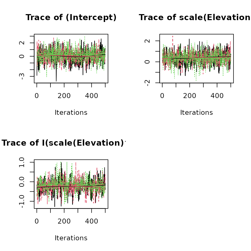
The summary() function does not present any information
on the latent factor loadings or latent factors, but the full posterior
samples are available in the lambda.samples and
w.samples tags in the out.lfMsPGOcc object,
respectively. Below we display the posterior summaries of the latent
factor loadings.
summary(out.lfMsPGOcc$lambda.samples)
Iterations = 1:1500
Thinning interval = 1
Number of chains = 1
Sample size per chain = 1500

1. Empirical mean and standard deviation for each variable,
   plus standard error of the mean:

            Mean     SD Naive SE Time-series SE
OVEN-1  1.000000 0.0000  0.00000        0.00000
BLPW-1 -0.882363 0.4511  0.01165        0.02217
AMRE-1 -0.637875 0.7588  0.01959        0.05350
BAWW-1  0.024814 0.7766  0.02005        0.05943
BHVI-1 -1.716477 0.6326  0.01633        0.04218
BLBW-1 -0.067492 0.6211  0.01604        0.05822
BTBW-1  1.496820 0.4924  0.01271        0.02859
BTNW-1  1.021993 0.4880  0.01260        0.03120
CAWA-1 -0.645987 0.5674  0.01465        0.04594
MAWA-1 -1.932342 0.5223  0.01349        0.03154
NAWA-1 -1.657577 0.6200  0.01601        0.04169
REVI-1  0.731117 0.4818  0.01244        0.03350
OVEN-2  0.000000 0.0000  0.00000        0.00000
BLPW-2  1.000000 0.0000  0.00000        0.00000
AMRE-2  0.008694 1.0353  0.02673        0.12548
BAWW-2  0.001111 0.9166  0.02367        0.08514
BHVI-2  0.226287 0.8916  0.02302        0.08868
BLBW-2  0.189532 1.0451  0.02698        0.12456
BTBW-2 -0.201146 0.6622  0.01710        0.04808
BTNW-2 -0.079416 0.9649  0.02491        0.10007
CAWA-2 -0.225772 0.9260  0.02391        0.10478
MAWA-2  0.160195 0.6962  0.01798        0.07025
NAWA-2  0.012736 0.9140  0.02360        0.11989
REVI-2  0.071562 0.7949  0.02052        0.07954

2. Quantiles for each variable:

          2.5%     25%        50%     75%    97.5%
OVEN-1  1.0000  1.0000  1.000e+00  1.0000  1.00000
BLPW-1 -1.7738 -1.1818 -8.703e-01 -0.5789 -0.03538
AMRE-1 -2.1539 -1.1327 -6.248e-01 -0.1693  0.94785
BAWW-1 -1.5394 -0.4532  6.063e-02  0.5014  1.49338
BHVI-1 -2.9867 -2.1184 -1.722e+00 -1.3356 -0.34155
BLBW-1 -1.4868 -0.4116 -4.060e-02  0.2989  1.11847
BTBW-1  0.6056  1.1460  1.486e+00  1.8326  2.49709
BTNW-1  0.1507  0.6859  9.871e-01  1.3286  2.09466
CAWA-1 -1.9103 -0.9899 -6.086e-01 -0.2511  0.41199
MAWA-1 -3.0176 -2.2753 -1.890e+00 -1.5646 -1.03734
NAWA-1 -3.0121 -2.0421 -1.616e+00 -1.2145 -0.57469
REVI-1 -0.1109  0.3913  6.897e-01  1.0115  1.78439
OVEN-2  0.0000  0.0000  0.000e+00  0.0000  0.00000
BLPW-2  1.0000  1.0000  1.000e+00  1.0000  1.00000
AMRE-2 -2.0837 -0.7007  3.519e-05  0.7192  2.06135
BAWW-2 -1.7059 -0.6712  3.792e-03  0.6437  1.80803
BHVI-2 -1.7020 -0.3498  2.549e-01  0.8181  1.95112
BLBW-2 -1.9739 -0.4545  2.906e-01  0.9197  1.99340
BTBW-2 -1.4853 -0.6514 -2.150e-01  0.2411  1.11520
BTNW-2 -2.0424 -0.6893 -5.008e-02  0.5353  1.81312
CAWA-2 -2.1012 -0.8626 -2.003e-01  0.4129  1.59162
MAWA-2 -1.2693 -0.3094  1.727e-01  0.6293  1.53020
NAWA-2 -1.7374 -0.6092 -7.732e-03  0.6351  1.83879
REVI-2 -1.4076 -0.4847  6.178e-02  0.5960  1.72262
The latent factor loadings and latent factors can provide information on the additional environmental drivers of species occurrence patterns, and what species are respondingly similarly to these environmental gradients. See Appendix S2 in Doser, Finley, and Banerjee (2023) for an example using North American Breeding Bird Survey data.
As previously discussed, determining the number of factors to include
in the model is not straightforward. However, looking at the posterior
summaries of the latent factor loadings can provide information on how
many factors are necessary for the given data set. In particular, we can
look at the posterior mean or median of the latent factor loadings for
each factor. If the factor loadings for all species are very close to
zero for a given factor, that suggests that factor is not an important
driver of species-specific occurrence across space, and thus you may
consider removing it from the model. Additionally, we can look at the
95% credible intervals, and if the 95% credible intervals for the factor
loadings of all species for a specific factor all contain zero this is
further support to reduce the number of factors in the model. In our
HBEF example, we see the factor loadings for the second factor for all
species are very close to zero, and zero is contained in all 95%
credible intervals. On the other hand, the estimated factor loadings for
the first factor range from significantly positive to significantly
negative values for different species, indicating it is an important
driver of occurrence across space. Given these findings, we refit the
model below with only a single latent factor. Note also that we fit the
model with default initial values and priors, and when we set
verbose = TRUE this information is clearly printed out to
the screen.
# Use default initial values and priors
# Approx. run time: 75 seconds
out.lfMsPGOcc.2 <- lfMsPGOcc(occ.formula = occ.formula, det.formula = det.formula,
                             data = hbef.ordered, n.factors = 1, n.samples = n.samples,
                             n.omp.threads = 1, verbose = TRUE, n.report = 1000,
                             n.burn = n.burn, n.thin = n.thin, n.chains = n.chains)
----------------------------------------
Preparing to run the model
----------------------------------------No prior specified for beta.comm.normal.
Setting prior mean to 0 and prior variance to 2.72No prior specified for alpha.comm.normal.
Setting prior mean to 0 and prior variance to 2.72No prior specified for tau.sq.beta.ig.
Setting prior shape to 0.1 and prior scale to 0.1No prior specified for tau.sq.alpha.ig.
Setting prior shape to 0.1 and prior scale to 0.1z is not specified in initial values.
Setting initial values based on observed databeta.comm is not specified in initial values.
Setting initial values to random values from the prior distributionalpha.comm is not specified in initial values.
Setting initial values to random values from the prior distributiontau.sq.beta is not specified in initial values.
Setting initial values to random values between 0.5 and 10tau.sq.alpha is not specified in initial values.
Setting initial values to random values between 0.5 and 10beta is not specified in initial values.
Setting initial values to random values from the community-level normal distributionalpha is not specified in initial values.
Setting initial values to random values from the community-level normal distributionlambda is not specified in initial values.
Setting initial values of the lower triangle to random values from a standard normal----------------------------------------
Model description
----------------------------------------
Latent Factor Multi-species Occupancy Model with Polya-Gamma latent
variable fit with 373 sites and 12 species.
Samples per Chain: 5000
Burn-in: 1000
Thinning Rate: 8
Number of Chains: 3
Total Posterior Samples: 1500
Using 1 latent factors.
Source compiled with OpenMP support and model fit using 1 thread(s).
----------------------------------------
Chain 1
----------------------------------------
Sampling ...
Sampled: 1000 of 5000, 20.00%
-------------------------------------------------
Sampled: 2000 of 5000, 40.00%
-------------------------------------------------
Sampled: 3000 of 5000, 60.00%
-------------------------------------------------
Sampled: 4000 of 5000, 80.00%
-------------------------------------------------
Sampled: 5000 of 5000, 100.00%
----------------------------------------
Chain 2
----------------------------------------
Sampling ...
Sampled: 1000 of 5000, 20.00%
-------------------------------------------------
Sampled: 2000 of 5000, 40.00%
-------------------------------------------------
Sampled: 3000 of 5000, 60.00%
-------------------------------------------------
Sampled: 4000 of 5000, 80.00%
-------------------------------------------------
Sampled: 5000 of 5000, 100.00%
----------------------------------------
Chain 3
----------------------------------------
Sampling ...
Sampled: 1000 of 5000, 20.00%
-------------------------------------------------
Sampled: 2000 of 5000, 40.00%
-------------------------------------------------
Sampled: 3000 of 5000, 60.00%
-------------------------------------------------
Sampled: 4000 of 5000, 80.00%
-------------------------------------------------
Sampled: 5000 of 5000, 100.00%Posterior Predictive Checks
The spOccupancy function ppcOcc() performs
a posterior predictive check for all spOccupancy model
objects as an assessment of Goodness of Fit (GoF). The key idea of GoF
testing is that a good model should generate data that closely align
with the observed data. If there are large differences in the observed
data from the model-generated data, our model is likely not very useful
(Hooten and Hobbs 2015). We can use the
ppcOcc() and summary() functions to generate a
Bayesian p-value as a quick assessment of model fit. A Bayesian p-value
that hovers around 0.5 indicates adequate model fit, while values less
than 0.1 or greater than 0.9 suggest our model does not fit the data
well. ppcOcc will return an overall Bayesian p-value for
the entire community, as well as an individual Bayesian p-value for each
species. See the
introductory spOccupancy vignette and the
ppcOcc() help page for additional details. Below we perform
a posterior predictive check with the Freeman-Tukey statistic, grouping
the data by individual sites.
# Approx run time: 30 seconds
ppc.out <- ppcOcc(out.lfMsPGOcc.2, fit.stat = 'freeman-tukey', group = 1)
Currently on species 1 out of 12Currently on species 2 out of 12Currently on species 3 out of 12Currently on species 4 out of 12Currently on species 5 out of 12Currently on species 6 out of 12Currently on species 7 out of 12Currently on species 8 out of 12Currently on species 9 out of 12Currently on species 10 out of 12Currently on species 11 out of 12Currently on species 12 out of 12
# Calculate Bayesian p-values
summary(ppc.out)
Call:
ppcOcc(object = out.lfMsPGOcc.2, fit.stat = "freeman-tukey",
    group = 1)

Samples per Chain: 5000
Burn-in: 1000
Thinning Rate: 8
Number of Chains: 3
Total Posterior Samples: 1500

----------------------------------------
    Community Level
----------------------------------------
Bayesian p-value:  0.4933

----------------------------------------
    Species Level
----------------------------------------
OVEN Bayesian p-value: 0.3673
BLPW Bayesian p-value: 0.644
AMRE Bayesian p-value: 0.5893
BAWW Bayesian p-value: 0.6693
BHVI Bayesian p-value: 0.8627
BLBW Bayesian p-value: 0.2547
BTBW Bayesian p-value: 0.58
BTNW Bayesian p-value: 0.2633
CAWA Bayesian p-value: 0.29
MAWA Bayesian p-value: 0.464
NAWA Bayesian p-value: 0.4747
REVI Bayesian p-value: 0.46
Fit statistic:  freeman-tukey
Here, our overall Bayesian p-value for the full community is close to 0.5, and the individual species Bayesian p-values also indicate adequate model fit.
Model Selection using WAIC
The spOccupancy function waicOCC()
calculates the Widely Applicable Information Criterion (Watanabe 2010) for all spOccupancy
fitted model objects. The WAIC is a useful fully Bayesian information
criterion that is adequate for comparing a set of hierarchical models
and selecting the best-performing model for final analysis (see the
introductory spOccupancy vignette for further details
on WAIC implementation in spOccupancy). Smaller values of
WAIC indicate a better performing model. Below, we fit a multi-species
occupancy model without species correlations using the
msPGOcc() function, and subsequently compare the model to
the model that does account for species correlations. Syntax for the
msPGOcc() function is identical to that for
lfMsPGOcc(), with the exception of the
n.factors argument no longer being included (since species
correlations are not accommodated).
# Approx run time: 71 seconds
out.msPGOcc <- msPGOcc(occ.formula = occ.formula, det.formula = det.formula,
                       data = hbef.ordered, inits = inits, priors = priors,
                       n.samples = n.samples, n.omp.threads = 1,
                       verbose = TRUE, n.report = 1000, n.burn = n.burn,
                       n.thin = n.thin, n.chains = n.chains)
----------------------------------------
Preparing to run the model
----------------------------------------
----------------------------------------
Model description
----------------------------------------
Multi-species Occupancy Model with Polya-Gamma latent
variable fit with 373 sites and 12 species.
Samples per Chain: 5000
Burn-in: 1000
Thinning Rate: 8
Number of Chains: 3
Total Posterior Samples: 1500
Source compiled with OpenMP support and model fit using 1 thread(s).
----------------------------------------
Chain 1
----------------------------------------
Sampling ...
Sampled: 1000 of 5000, 20.00%
-------------------------------------------------
Sampled: 2000 of 5000, 40.00%
-------------------------------------------------
Sampled: 3000 of 5000, 60.00%
-------------------------------------------------
Sampled: 4000 of 5000, 80.00%
-------------------------------------------------
Sampled: 5000 of 5000, 100.00%
----------------------------------------
Chain 2
----------------------------------------
Sampling ...
Sampled: 1000 of 5000, 20.00%
-------------------------------------------------
Sampled: 2000 of 5000, 40.00%
-------------------------------------------------
Sampled: 3000 of 5000, 60.00%
-------------------------------------------------
Sampled: 4000 of 5000, 80.00%
-------------------------------------------------
Sampled: 5000 of 5000, 100.00%
----------------------------------------
Chain 3
----------------------------------------
Sampling ...
Sampled: 1000 of 5000, 20.00%
-------------------------------------------------
Sampled: 2000 of 5000, 40.00%
-------------------------------------------------
Sampled: 3000 of 5000, 60.00%
-------------------------------------------------
Sampled: 4000 of 5000, 80.00%
-------------------------------------------------
Sampled: 5000 of 5000, 100.00%
# Compute WAIC for the the latent factor multi-species occupancy model.
waicOcc(out.lfMsPGOcc.2)
elpd pD WAIC
-4354.6047 184.8315 9078.8723
# Compute WAIC for the basic multi-species occupancy model.
waicOcc(out.msPGOcc)
elpd pD WAIC
-4531.69679 65.77426 9194.94210 Here, we see the WAIC for the latent factor multi-species occupancy model is substantially lower than the WAIC for the multi-species occupancy model, suggesting that accommodating residual species correlations leads to improved model performance in the foliage-gleaning bird data set.
As of v0.7.0, waicOcc() contains the
by.sp argument, which allows us to calculate the WAIC
separately for each species by setting by.sp = TRUE. Note
that the WAIC values for each individual species sum to the total
overall WAIC value for the model
waicOcc(out.lfMsPGOcc.2, by.sp = TRUE) elpd pD WAIC
1 -600.42735 21.851344 1244.55739
2 -132.48462 10.079209 285.12765
3 -24.95701 2.869529 55.65307
4 -176.25601 5.959846 364.43172
5 -228.99376 15.872065 489.73165
6 -702.99327 10.802212 1427.59097
7 -668.49488 29.103013 1395.19578
8 -714.75286 20.018258 1469.54225
9 -104.31410 8.875385 226.37898
10 -222.48305 30.097801 505.16170
11 -89.82531 15.334373 210.31936
12 -688.62246 13.968430 1405.18178
waicOcc(out.msPGOcc, by.sp = TRUE) elpd pD WAIC
1 -632.90106 5.897659 1277.59743
2 -139.46066 5.047269 289.01585
3 -26.10348 2.183308 56.57358
4 -176.55409 5.322369 363.75292
5 -247.30402 3.901586 502.41122
6 -705.03130 7.646545 1425.35569
7 -699.32967 6.900581 1412.46050
8 -730.74286 6.732369 1474.95045
9 -107.92878 4.885538 225.62864
10 -261.86341 5.511024 534.74887
11 -106.72691 5.445612 224.34504
12 -697.75056 6.300399 1408.10191Prediction
Finally, we can use the predict() function with all
spOccupancy model-fitting functions to generate a series of
posterior predictive samples at new locations, given a set of covariates
and their spatial locations. spOccupancy supports
prediction of both new occurrence values at a set of spatial locations
and as of v0.3.0, spOccupancy supports predictions of
detection probability over a range of covariate values.
First, we show how to use predict() to create a map of
species richness across HBEF. The object hbefElev (which
comes as part of the spOccupancy package) contains
elevation data at a 30x30m resolution from the National Elevation
Dataset across the entire HBEF. We load the data below.
'data.frame': 46090 obs. of 3 variables:
$ val : num 914 916 918 920 922 ...
$ Easting : num 276273 276296 276318 276340 276363 ...
$ Northing: num 4871424 4871424 4871424 4871424 4871424 ...The column val contains the elevation values, while
Easting and Northing contain the spatial
coordinates of the prediction sites. Below we standardize our new
elevation values using the mean and standard deviation of the elevation
values we used to fit the data, and then predict occurrence for each
species across all 46090 spatial locations. The out.pred
object consists of posterior predictive samples of the latent occurrence
probability (psi.0.samples) as well as the latent
occurrence state (z.0.samples). We can calculate species
richness as a derived quantity by summing up the latent occurrence
states for each species at each MCMC sample.
# Not run (note this takes a large amount of memory to run).
elev.pred <- (hbefElev$val - mean(hbef2015$occ.covs[, 1])) / sd(hbef2015$occ.covs[, 1])
# Order: intercept, elevation (linear), elevation (quadratic)
X.0 <- cbind(1, elev.pred, elev.pred^2)
# Spatial coordinates
coords.0 <- as.matrix(hbefElev[, c('Easting', 'Northing')])
# type = 'occupancy' specifies prediction of occupancy (or occurrence).
# This is also the default.
# Approximate run time: 30 sec
out.pred <- predict(out.lfMsPGOcc, X.0, coords.0, type = 'occupancy')
str(out.pred)
# Species richness samples
rich.pred <- apply(out.pred$z.0.samples, c(1, 3), sum)
plot.dat <- data.frame(x = hbefElev$Easting,
y = hbefElev$Northing,
rich.mean = apply(rich.pred, 2, mean),
rich.sd = apply(rich.pred, 2, sd))
# Plot species richness of the foliage-gleaning bird community
# across the Hubbard Brook Experimental Forest
dat.stars <- st_as_stars(plot.dat, dims = c('x', 'y'))
ggplot() +
geom_stars(data = dat.stars, aes(x = x, y = y, fill = rich.mean)) +
scale_fill_viridis_c(na.value = 'transparent') +
labs(x = 'Easting', y = 'Northing', fill = '',
title = 'Mean Species Richness') +
theme_bw()Note that when predicting new values using a latent factor
multi-species occupancy model (or a latent factor joint species
distribution model as we will see with lfJSDM()), we make
predictions at both sampled and non-sampled locations using the latent
factors. At sampled locations, we directly use the posterior samples
from the model fit in the prediction algorithm, which will generally
lead to improved predictions at the sampled sites compared to a
multi-species model that does not account for species correlations and
incorporate these factors. At non-sampled sites, we do not know the
value of the latent factors, and so we simply draw random values from a
standard normal distribution at each iteration of the posterior
predictive sampling algorithm. Because these values are drawn form a
normal distribution with a mean of 0, including these predictions of the
latent factors at new sites will not change the overall mean estimate of
occurrence probability at that site, but it will account for the
uncertainty we have in the latent factor values, and thus will fully
propagate uncertainty from our model fit to the resulting
predictions.
Finally, we can generate predicted values of detection probability across a range of covariate values to generate a marginal response curve for each individual species across any given covariate value. Below we predict and plot the relationships between detection probability and time of day for each of the 12 species, while holding the day of the year at it’s mean value (0).
# Minimum observed time of day
min.tod <- min(hbef2015$det.covs$tod, na.rm = TRUE)
# Maximum
max.tod <- max(hbef2015$det.covs$tod, na.rm = TRUE)
# Generate 100 time of day values between the observed range
J.0 <- 100
tod.pred.vals <- seq(from = min.tod, to = max.tod, length.out = J.0)
# Standardize the new values by the mean and sd of the data
# used to fit the model.
mean.tod <- mean(hbef2015$det.covs$tod, na.rm = TRUE)
sd.tod <- sd(hbef2015$det.covs$tod, na.rm = TRUE)
tod.stand <- (tod.pred.vals - mean.tod) / sd.tod
# Generate covariate matrix for prediction
X.p.0 <- cbind(1, 0, tod.stand, 0)
colnames(X.p.0) <- c('intercept', 'day', 'tod', 'day2')
out.det.pred <- predict(out.lfMsPGOcc, X.p.0, type = 'detection')
str(out.det.pred)List of 2
$ p.0.samples: num [1:1500, 1:12, 1:100] 0.697 0.68 0.717 0.617 0.71 ...
$ call : language predict.lfMsPGOcc(object = out.lfMsPGOcc, X.0 = X.p.0, type = "detection")
- attr(*, "class")= chr "predict.lfMsPGOcc"The p.0.samples tag in the out.det.pred
object consists of the posterior predictive samples of detection
probability for each species across the 100 generated time of day
values. We finally create a marginal response curve for each species
using ggplot2.
# Extract the means from the posterior samples and convert to vector
p.0.ests <- c(apply(out.det.pred$p.0.samples, c(2, 3), mean))
p.plot.dat <- data.frame(det.prob = p.0.ests,
sp = rep(sp.names, J.0),
tod = rep(tod.pred.vals, each = N))
ggplot(p.plot.dat, aes(x = tod, y = det.prob)) +
geom_line() +
theme_bw() +
scale_y_continuous(limits = c(0, 1)) +
facet_wrap(vars(sp)) +
labs(x = 'Time of day (min since sunrise)', y = 'Detection Probability') 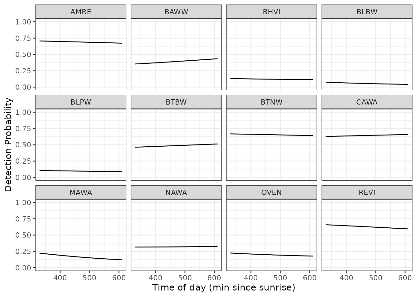
The relatively flat lines here for most species indicates that detection probability does not vary to a large extent across the time of day range that is sampled in the data, although there is some apparent variability in the effect across species (e.g., BAWW vs. MAWA).
Spatial factor multi-species occupancy models
Basic model description
While the latent factor multi-species occupancy model accounts for
species correlations and imperfect detection, it fails to address
spatial autocorrelation. The spatial factor multi-species occupancy
model is identical to the latent factor multi-species occupancy model
(lfMsPGOcc()), except the latent factors are now assumed to
arise from a spatial process rather than a standard normal distribution,
which accounts for spatial autocorrelation in latent species occurrence.
More specifically, each latent factor (now called a spatial factor)
\(\textbf{w}_r\) for each \(r = 1, \dots, q\) is modeled using a
Nearest Neighbor Gaussian Process (Datta et al.
2016), i.e.,
\[\begin{equation} \text{w}_r(\boldsymbol{s}_j) \sim N(\boldsymbol{0}, \tilde{\boldsymbol{C}}_r(\boldsymbol{\theta}_r)), \end{equation}\]
where \(\tilde{\boldsymbol{C}}_r(\boldsymbol{\theta}_r)\)
is the NNGP-derived covariance matrix for the \(r^{\text{th}}\) spatial factor. The vector
\(\boldsymbol{\theta}_r\) consists of
parameters governing the spatial process according to a spatial
correlation function (Banerjee, Carlin, and
Gelfand 2014). spOccupancy implements four spatial
correlation functions: exponential, spherical, Gaussian, and Matern. For
the exponential, spherical, and Gaussian functions, \(\boldsymbol{\theta}_r\) includes a spatial
variance parameter, \(\sigma^2_r\), and
a spatial range parameter, \(\phi_r\),
while the Matern correlation function includes an additional spatial
smoothness parameter, \(\nu_r\).
We assume the same priors and identifiability constraints as the latent factor multi-species occupancy model. We assign a uniform prior the spatial range parameters, \(\phi_r\), and the spatial smoothness parameters, \(\nu_r\), if using a Matern correlation function.
Fitting spatial factor multi-species occupancy models with
sfMsPGOcc
The function sfMsPGOcc() fits spatial factor
multi-species occupancy models using Pólya-Gamma data augmentation.
sfMsPGOcc() has the following arguments:
sfMsPGOcc(occ.formula, det.formula, data, inits, priors,
tuning, cov.model = 'exponential', NNGP = TRUE,
n.neighbors = 15, search.type = "cb", n.factors,
n.batch, batch.length, accept.rate = 0.43,
n.omp.threads = 1, verbose = TRUE, n.report = 100,
n.burn = round(.10 * n.batch * batch.length),
n.thin = 1, n.chains = 1, k.fold, k.fold.threads = 1,
k.fold.seed = 100, k.fold.only = FALSE, ...){We will walk through each of the arguments to
sfMsPGOcc() in the context of our HBEF example. The
occurrence (occ.formula) and detection
(det.formula) formulas, as well as the list of data
(data) follow the same form as we saw in
lfMsPGOcc(). We will specify these again below for
clarity.
occ.formula <- ~ scale(Elevation) + I(scale(Elevation)^2)
det.formula <- ~ scale(day) + scale(tod) + I(scale(day)^2)
# Remind ourselves what the data look like
str(hbef.ordered)List of 4
$ y : num [1:12, 1:373, 1:3] 1 0 0 0 0 0 1 0 0 0 ...
..- attr(*, "dimnames")=List of 3
.. ..$ : chr [1:12] "OVEN" "BLPW" "AMRE" "BAWW" ...
.. ..$ : chr [1:373] "1" "2" "3" "4" ...
.. ..$ : chr [1:3] "1" "2" "3"
$ occ.covs: num [1:373, 1] 475 494 546 587 588 ...
..- attr(*, "dimnames")=List of 2
.. ..$ : NULL
.. ..$ : chr "Elevation"
$ det.covs:List of 2
..$ day: num [1:373, 1:3] 156 156 156 156 156 156 156 156 156 156 ...
..$ tod: num [1:373, 1:3] 330 346 369 386 409 425 447 463 482 499 ...
$ coords : num [1:373, 1:2] 280000 280000 280000 280001 280000 ...
..- attr(*, "dimnames")=List of 2
.. ..$ : chr [1:373] "1" "2" "3" "4" ...
.. ..$ : chr [1:2] "X" "Y"Following our findings from using lfMsPGOcc(), we will
use 1 latent spatial factor.
n.factors <- 1We will next specify the initial values in the inits
argument. Just as before, this argument is optional as
spOccupancy will by default set the initial values based on
the prior distributions. Valid tags for initial values include all the
parameters described for the latent factor multi-species occupancy model
using lfMsPGOcc() as well as parameters associated with the
spatial latent processes. These include: phi (the spatial
range parameter) and nu (the spatial smoothness parameter),
where the latter is only specified if adopting a Matern covariance
function (i.e., cov.model = 'matern').
spOccupancy supports four spatial covariance models
(exponential, spherical,
gaussian, and matern), which are specified in
the cov.model argument. Here we will use an exponential
correlation function. When using an exponential correlation function,
\(\frac{3}{\phi}\) is the effective
range, or the distance at which the residual spatial correlation between
two sites drops to 0.05 (Banerjee, Carlin, and
Gelfand 2014). As an initial value for the spatial range
parameter phi, we compute the mean distance between points
in HBEF and then set it equal to 3 divided by this mean distance. Thus,
our initial guess for the effective range is the average distance
between sites across HBEF. We will set all other initial values to the
same values we used for lfMsPGOcc().
# Pair-wise distance between all sites
dist.hbef <- dist(hbef.ordered$coords)
# Exponential correlation model
cov.model <- "exponential"
# Specify all other initial values identical to lfMsPGOcc() from before
# Number of species
N <- nrow(hbef.ordered$y)
# Initiate all lambda initial values to 0.
lambda.inits <- matrix(0, N, n.factors)
# Set diagonal elements to 1
diag(lambda.inits) <- 1
# Set lower triangular elements to random values from a standard normal dist
lambda.inits[lower.tri(lambda.inits)] <- rnorm(sum(lower.tri(lambda.inits)))
# Check it out
lambda.inits [,1]
[1,] 1.00000000
[2,] 0.08726913
[3,] 1.04191535
[4,] -0.57058400
[5,] -1.03868418
[6,] 0.57980601
[7,] -0.91943441
[8,] 1.54189049
[9,] 0.39333145
[10,] 1.75861735
[11,] 2.15505834
[12,] 0.11110001
# Create list of initial values.
inits <- list(alpha.comm = 0,
beta.comm = 0,
beta = 0,
alpha = 0,
tau.sq.beta = 1,
tau.sq.alpha = 1,
lambda = lambda.inits,
phi = 3 / mean(dist.hbef),
z = apply(hbef.ordered$y, c(1, 2), max, na.rm = TRUE))The next three arguments (n.batch,
batch.length, and accept.rate) are all related
to the Adaptive MCMC sampler used when we fit the model. Updates for the
spatial range parameter (and the smoothness parameter if
cov.model = 'matern') require the use of a
Metropolis-Hastings algorithm. We implement an adaptive
Metropolis-Hastings algorithm as discussed in Roberts and Rosenthal (2009). This algorithm
adjusts the tuning values for each parameter that requires a
Metropolis-Hastings update within the sampler itself. This process
results in a more efficient sampler than if we were to fix the tuning
parameters prior to fitting the model. The parameter
accept.rate is the target acceptance rate for each
parameter, and the algorithm will adjust the tuning parameters to hover
around this value. The default value is 0.43, which we suggest leaving
as is unless you have a good reason to change it. The tuning parameters
are updated after a single “batch”. In lfMsPGOcc(), we
specified an n.samples argument which consisted of the
total number of samples to run each chain of the MCMC. For
sfMsPGOcc() (and all spatially-explicit models in
spOccupancy), we break up the total number of MCMC samples
into a set of “batches”, where each batch has a specific number of
samples. We must specify both the total number of batches
(n.batch) as well as the number of MCMC samples each batch
contains (batch.length). Thus, the total number of MCMC
samples is n.batch * batch.length. Typically, we set
batch.length = 25 and then play around with
n.batch until convergence is reached. We recommend keeping
this at 25 unless you have a specific reason to change it. Here we set
n.batch = 200 for a total of 5000 MCMC samples in each of 3
chains. We will additionally specify a burn-in period of length 3000 and
a thinning rate of 2. Importantly, we also need to specify an initial
value for the tuning parameters for the spatial decay and smoothness
parameters (if applicable). These values are supplied as input in the
form of a list with tags phi and nu. The
initial tuning value can be any value greater than 0, but we recommend
starting the value out around 0.5. After some initial runs of the model,
if you notice the final acceptance rate of a parameter is much larger or
smaller than the target acceptance rate (accept.rate), you
can then change the initial tuning value to get closer to the target
rate. Here we set the initial tuning value for phi to 1
after some initial exploratory runs of the model.
batch.length <- 25
n.batch <- 200
n.burn <- 3000
n.thin <- 2
n.chains <- 3Priors are again specified in a list in the priors
argument. We assume uniform priors for the spatial decay parameter
phi and smoothness parameter nu (if using the
Matern correlation function), with the associated tags
phi.unif and nu.unif. The lower and upper
bounds of the uniform distribution are passed as a two-element vector
for the uniform priors.
Here we use an exponential correlation function, so we only need to
specify priors for the spatial decay parameter phi for each
of the spatial factors (which in this case is just 1). We recommend
determining the bounds of the uniform distribution by computing the
smallest distance between sites and the largest distance between sites
in the observed data set. We then set the lower bound of the uniform to
3/max and the upper bound to 3/min, where
min and max correspond to the predetermined
distances between sites. This equates to a vague prior that states that
spatial autocorrelation in the spatial factors could only be between
sites that are very close to each other, or could span across the entire
observed study area. We recommend using these bounds for the prior
unless you have prior information about the range of the spatial
autocorrelation. The remaining priors are identical to what we saw in
lfMsPGOcc(). We use the same priors for all other
parameters as those we used for lfMsPGOcc().
min.dist <- min(dist.hbef)
max.dist <- max(dist.hbef)
priors <- list(beta.comm.normal = list(mean = 0, var = 2.72),
alpha.comm.normal = list(mean = 0, var = 2.72),
tau.sq.beta.ig = list(a = 0.1, b = 0.1),
tau.sq.alpha.ig = list(a = 0.1, b = 0.1),
phi.unif = list(3 / max.dist, 3 / min.dist))Importantly, we also need to specify an initial value for the tuning
parameters for the spatial decay and smoothness parameters (if
applicable). These values are supplied as input in the form of a list
with tags phi and nu. The initial tuning value
can be any value greater than 0, but we recommend starting the value out
around 0.5. After some initial runs of the model, if you notice the
final acceptance rate of a parameter is much larger or smaller than the
target acceptance rate (accept.rate), you can then change
the initial tuning value to get closer to the target rate. Here we set
the initial tuning value for phi to 1 after some initial
exploratory runs of the model.
tuning <- list(phi = 1)The argument n.omp.threads specifies the number of
threads to use for within-chain parallelization, which can greatly
decrease run time for spatially-explicit models (Andrew O. Finley, Datta, and Banerjee 2020),
while verbose specifies whether or not to print the
progress of the sampler. We highly recommend setting
verbose = TRUE for all spatial models to ensure the
adaptive MCMC is working as you want (and this is the reason for why
this is the default for this argument). The argument
n.report specifies the interval to report the
Metropolis-Hastings sampler acceptance rate. Note that
n.report is specified in terms of batches, not the overall
number of samples. Below we set n.report = 50, which will
result in information on the acceptance rate and tuning parameters every
50th batch (not sample). Ideally, you should see the printed acceptance
rate values however around the value supplied to the
accept.rate argument (which by default is 0.43). If by the
end of the MCMC run you see the values are well below the target
acceptance rate, we recommend rerunning the model with a larger initial
tuning parameter (higher than the final reported value in the displayed
output of model progress). If you see the values are well above the
target acceptance rate, we recommend rerunning the model with a smaller
initial tuning parameter (smaller than the final reported value).
n.omp.threads <- 1
verbose <- TRUE
n.report <- 50 # Report progress at every 50th batch.The parameters NNGP, n.neighbors, and
search.type relate to whether or not you want to fit the
model with a Gaussian Process or with NNGP, which is a much more
computationally efficient approximation. The argument NNGP
is a logical value indicating whether to fit the model with an NNGP
(TRUE) or a regular Gaussian Process (FALSE).
Currently, sfMsPGOcc() only supports NNGP models, so you
will receive an error message if you set NNGP = FALSE that
tells you to switch to NNGP = TRUE. We plan to implement
these models with a full Gaussian Process in future development. The
argument n.neighbors and search.type specify
the number of neighbors used in the NNGP and the nearest neighbor search
algorithm, respectively, to use for the NNGP model. Generally, the
default values of these arguments will be adequate. Datta et al. (2016) showed that setting
n.neighbors = 15 is usually sufficient, although for
certain data sets a good approximation can be achieved with as few as
five neighbors, which could substantially decrease run time for the
model. We generally recommend leaving search.type = "cb",
as this results in a fast code book nearest neighbor search algorithm.
However, details on when you may want to change this are described in
Andrew O. Finley, Datta, and Banerjee
(2020). We will run an NNGP model using the default value for
search.type and setting n.neighbors = 5. Here
we choose 5 neighbors because we found in Doser,
Finley, et al. (2022) that estimates from a spatial multi-species
occupancy model for this data set were relatively robust to the number
of neighbors in the model. Generally, we recommend using the default
value of n.neighbors = 15, and if additional decreases in
computation time are desired, you can fit the model with
n.neighbors = 5 and compare their performance using WAIC
and/or k-fold cross-validation.
We now fit the model using sfMsPGOcc() and summarize the
results using summary().
# Approx run time: 2 min
out.sfMsPGOcc <- sfMsPGOcc(occ.formula = occ.formula,
det.formula = det.formula,
data = hbef.ordered,
inits = inits,
n.batch = n.batch,
batch.length = batch.length,
accept.rate = 0.43,
priors = priors,
n.factors = n.factors,
cov.model = cov.model,
tuning = tuning,
n.omp.threads = n.omp.threads,
verbose = TRUE,
NNGP = TRUE,
n.neighbors = 5,
n.report = n.report,
n.burn = n.burn,
n.thin = n.thin,
n.chains = n.chains)----------------------------------------
Preparing to run the model
----------------------------------------
----------------------------------------
Building the neighbor list
----------------------------------------
----------------------------------------
Building the neighbors of neighbors list
----------------------------------------
----------------------------------------
Model description
----------------------------------------
Spatial Factor NNGP Multi-species Occupancy Model with Polya-Gamma latent
variable fit with 373 sites and 12 species.
Samples per chain: 5000 (200 batches of length 25)
Burn-in: 3000
Thinning Rate: 2
Number of Chains: 3
Total Posterior Samples: 3000
Using the exponential spatial correlation model.
Using 1 latent spatial factors.
Using 5 nearest neighbors.
Source compiled with OpenMP support and model fit using 1 thread(s).
Adaptive Metropolis with target acceptance rate: 43.0
----------------------------------------
Chain 1
----------------------------------------
Sampling ...
Batch: 50 of 200, 25.00%
Latent Factor Parameter Acceptance Tuning
1 phi 16.0 0.60050
-------------------------------------------------
Batch: 100 of 200, 50.00%
Latent Factor Parameter Acceptance Tuning
1 phi 20.0 0.37908
-------------------------------------------------
Batch: 150 of 200, 75.00%
Latent Factor Parameter Acceptance Tuning
1 phi 52.0 0.29820
-------------------------------------------------
Batch: 200 of 200, 100.00%
----------------------------------------
Chain 2
----------------------------------------
Sampling ...
Batch: 50 of 200, 25.00%
Latent Factor Parameter Acceptance Tuning
1 phi 52.0 0.28083
-------------------------------------------------
Batch: 100 of 200, 50.00%
Latent Factor Parameter Acceptance Tuning
1 phi 48.0 0.28083
-------------------------------------------------
Batch: 150 of 200, 75.00%
Latent Factor Parameter Acceptance Tuning
1 phi 40.0 0.29820
-------------------------------------------------
Batch: 200 of 200, 100.00%
----------------------------------------
Chain 3
----------------------------------------
Sampling ...
Batch: 50 of 200, 25.00%
Latent Factor Parameter Acceptance Tuning
1 phi 52.0 0.27527
-------------------------------------------------
Batch: 100 of 200, 50.00%
Latent Factor Parameter Acceptance Tuning
1 phi 32.0 0.26982
-------------------------------------------------
Batch: 150 of 200, 75.00%
Latent Factor Parameter Acceptance Tuning
1 phi 28.0 0.25924
-------------------------------------------------
Batch: 200 of 200, 100.00%
# Take a look at the resulting object
names(out.sfMsPGOcc) [1] "rhat" "beta.comm.samples" "alpha.comm.samples"
[4] "tau.sq.beta.samples" "tau.sq.alpha.samples" "beta.samples"
[7] "alpha.samples" "lambda.samples" "theta.samples"
[10] "z.samples" "w.samples" "psi.samples"
[13] "like.samples" "X.p" "X.p.re"
[16] "X.re" "ESS" "X"
[19] "y" "call" "n.samples"
[22] "x.names" "sp.names" "x.p.names"
[25] "theta.names" "type" "coords"
[28] "cov.model.indx" "n.neighbors" "q"
[31] "n.post" "n.thin" "n.burn"
[34] "n.chains" "pRE" "psiRE"
[37] "std.by.sp" "species.sds" "species.means"
[40] "run.time"
summary(out.sfMsPGOcc)
Call:
sfMsPGOcc(occ.formula = occ.formula, det.formula = det.formula,
data = hbef.ordered, inits = inits, priors = priors, tuning = tuning,
cov.model = cov.model, NNGP = TRUE, n.neighbors = 5, n.factors = n.factors,
n.batch = n.batch, batch.length = batch.length, accept.rate = 0.43,
n.omp.threads = n.omp.threads, verbose = TRUE, n.report = n.report,
n.burn = n.burn, n.thin = n.thin, n.chains = n.chains)
Samples per Chain: 5000
Burn-in: 3000
Thinning Rate: 2
Number of Chains: 3
Total Posterior Samples: 3000
Run Time (min): 0.9862
----------------------------------------
Community Level
----------------------------------------
Occurrence Means (logit scale):
Mean SD 2.5% 50% 97.5% Rhat ESS
(Intercept) 0.4138 0.9397 -1.4779 0.3957 2.3251 1.2572 305
scale(Elevation) 0.4409 0.5785 -0.6575 0.4315 1.6466 1.0221 694
I(scale(Elevation)^2) -0.2005 0.3121 -0.8185 -0.2045 0.4300 1.0172 507
Occurrence Variances (logit scale):
Mean SD 2.5% 50% 97.5% Rhat ESS
(Intercept) 15.3672 8.9701 5.2263 13.1667 37.3060 1.1911 194
scale(Elevation) 4.1324 2.8989 1.2564 3.4288 11.5424 1.0062 187
I(scale(Elevation)^2) 1.0268 0.7498 0.2302 0.8291 2.9140 1.0933 159
Detection Means (logit scale):
Mean SD 2.5% 50% 97.5% Rhat ESS
(Intercept) -0.8440 0.5077 -1.8520 -0.8361 0.1299 1.1440 655
scale(day) 0.0538 0.0865 -0.1116 0.0519 0.2276 1.0035 2085
scale(tod) -0.0402 0.0783 -0.2038 -0.0382 0.1106 1.0043 1746
I(scale(day)^2) -0.0245 0.0874 -0.2030 -0.0236 0.1471 1.0071 1849
Detection Variances (logit scale):
Mean SD 2.5% 50% 97.5% Rhat ESS
(Intercept) 3.2253 1.9799 0.9487 2.7714 8.0954 1.6838 91
scale(day) 0.0661 0.0392 0.0237 0.0565 0.1665 1.0074 2360
scale(tod) 0.0513 0.0330 0.0165 0.0425 0.1409 1.0033 1895
I(scale(day)^2) 0.0594 0.0418 0.0182 0.0486 0.1654 1.0049 2009
----------------------------------------
Species Level
----------------------------------------
Occurrence (logit scale):
Mean SD 2.5% 50% 97.5% Rhat ESS
(Intercept)-OVEN 2.2232 0.3314 1.5895 2.2180 2.8748 1.0701 177
(Intercept)-BLPW -5.7697 1.0465 -8.0832 -5.6610 -3.9472 1.0100 107
(Intercept)-AMRE 1.2309 4.6123 -4.2302 -0.2234 10.8491 6.3902 4
(Intercept)-BAWW 3.3036 1.9751 0.3983 3.0504 8.2504 1.6138 28
(Intercept)-BHVI 0.1886 0.7891 -1.2358 0.1418 1.8634 1.0618 94
(Intercept)-BLBW 2.6816 0.5819 1.7909 2.5941 4.0177 1.1033 233
(Intercept)-BTBW 4.8988 0.9606 3.3064 4.8145 7.0738 1.1175 83
(Intercept)-BTNW 2.7775 0.6249 1.9130 2.6695 4.2350 1.1857 93
(Intercept)-CAWA -1.9070 0.7719 -3.1182 -2.0276 -0.0458 1.4897 90
(Intercept)-MAWA -2.9031 0.6689 -4.2598 -2.8512 -1.6852 1.0923 122
(Intercept)-NAWA -2.9662 0.7356 -4.4512 -2.9766 -1.3863 1.0539 130
(Intercept)-REVI 3.2167 0.5093 2.3532 3.1647 4.3385 1.0479 252
scale(Elevation)-OVEN -1.7234 0.3096 -2.3872 -1.7024 -1.1968 1.0083 320
scale(Elevation)-BLPW 3.1076 0.8360 1.8207 2.9639 5.0454 1.1226 83
scale(Elevation)-AMRE 1.0788 1.3709 -1.8998 1.0092 3.8415 1.2556 38
scale(Elevation)-BAWW -1.0660 1.1156 -4.1174 -0.8335 0.4457 1.4923 45
scale(Elevation)-BHVI 0.5318 0.6454 -0.6206 0.4600 1.9835 1.0225 109
scale(Elevation)-BLBW -0.4785 0.2256 -0.9609 -0.4619 -0.0797 1.0268 512
scale(Elevation)-BTBW -0.4066 0.2933 -1.0163 -0.3921 0.1442 1.0263 186
scale(Elevation)-BTNW 0.7903 0.3206 0.2689 0.7513 1.5356 1.0517 272
scale(Elevation)-CAWA 2.4901 1.0073 1.0395 2.3054 4.9912 1.6194 61
scale(Elevation)-MAWA 2.4449 0.6415 1.3712 2.4044 3.8010 1.0154 124
scale(Elevation)-NAWA 1.1467 0.4250 0.4113 1.1183 2.0699 1.0113 258
scale(Elevation)-REVI -2.2433 0.7679 -4.0150 -2.1394 -1.0763 1.0355 86
I(scale(Elevation)^2)-OVEN -0.4673 0.2336 -0.9013 -0.4776 0.0200 1.0079 397
I(scale(Elevation)^2)-BLPW 1.0045 0.5287 -0.0138 0.9963 2.0751 1.0390 183
I(scale(Elevation)^2)-AMRE -0.8195 0.8992 -2.5996 -0.7959 1.0328 1.2683 57
I(scale(Elevation)^2)-BAWW -1.2670 0.6803 -2.6098 -1.2460 0.3018 1.6690 91
I(scale(Elevation)^2)-BHVI 0.6318 0.5286 -0.2078 0.5625 1.9148 1.0919 108
I(scale(Elevation)^2)-BLBW -0.5973 0.1854 -0.9983 -0.5924 -0.2655 1.0772 425
I(scale(Elevation)^2)-BTBW -1.3991 0.3022 -2.0297 -1.3830 -0.8683 1.0601 134
I(scale(Elevation)^2)-BTNW -0.2038 0.2099 -0.6486 -0.1993 0.1901 1.0110 246
I(scale(Elevation)^2)-CAWA -0.3640 0.6941 -1.6325 -0.4155 1.1594 1.2152 89
I(scale(Elevation)^2)-MAWA 0.6933 0.4285 -0.0979 0.6780 1.5865 1.0528 256
I(scale(Elevation)^2)-NAWA 0.3176 0.3450 -0.3511 0.3166 0.9757 1.0241 279
I(scale(Elevation)^2)-REVI 0.0477 0.4042 -0.6370 0.0156 0.9618 1.0113 124
Detection (logit scale):
Mean SD 2.5% 50% 97.5% Rhat ESS
(Intercept)-OVEN 0.8300 0.1164 0.6087 0.8260 1.0617 1.0031 2790
(Intercept)-BLPW -0.4649 0.2634 -0.9933 -0.4538 0.0274 1.0033 2029
(Intercept)-AMRE -3.8784 1.5851 -6.1965 -4.2629 -0.7433 4.1472 7
(Intercept)-BAWW -2.8206 0.3262 -3.4224 -2.8417 -2.1062 1.1753 75
(Intercept)-BHVI -2.2355 0.2699 -2.7663 -2.2290 -1.7087 1.0502 156
(Intercept)-BLBW -0.0464 0.1268 -0.3027 -0.0456 0.2008 1.0321 568
(Intercept)-BTBW 0.6366 0.1073 0.4288 0.6359 0.8542 1.0030 3000
(Intercept)-BTNW 0.5789 0.1133 0.3628 0.5772 0.8085 1.0040 1284
(Intercept)-CAWA -2.0038 0.6100 -3.0334 -2.0647 -0.8061 1.7153 47
(Intercept)-MAWA -0.7535 0.2118 -1.1669 -0.7552 -0.3235 1.0151 1100
(Intercept)-NAWA -1.5087 0.4549 -2.4288 -1.4964 -0.6260 1.1064 215
(Intercept)-REVI 0.5461 0.1089 0.3334 0.5456 0.7645 1.0006 2444
scale(day)-OVEN -0.0758 0.0740 -0.2247 -0.0746 0.0679 1.0025 3000
scale(day)-BLPW 0.0606 0.1553 -0.2413 0.0608 0.3704 1.0011 2751
scale(day)-AMRE 0.0262 0.2355 -0.4381 0.0250 0.4916 1.0044 1213
scale(day)-BAWW 0.2124 0.1417 -0.0597 0.2103 0.4976 1.0014 1276
scale(day)-BHVI 0.1884 0.1215 -0.0517 0.1850 0.4272 1.0086 1858
scale(day)-BLBW -0.2241 0.0677 -0.3617 -0.2226 -0.0929 1.0064 3000
scale(day)-BTBW 0.2702 0.0695 0.1330 0.2690 0.4039 1.0003 2660
scale(day)-BTNW 0.1464 0.0661 0.0163 0.1454 0.2758 1.0022 3000
scale(day)-CAWA -0.0218 0.1746 -0.3657 -0.0192 0.3250 1.0007 2156
scale(day)-MAWA 0.1064 0.1242 -0.1440 0.1053 0.3572 1.0072 2689
scale(day)-NAWA 0.0136 0.1770 -0.3505 0.0130 0.3610 1.0021 2373
scale(day)-REVI -0.0722 0.0677 -0.2047 -0.0725 0.0604 1.0069 3016
scale(tod)-OVEN -0.0413 0.0729 -0.1846 -0.0418 0.1037 1.0061 2723
scale(tod)-BLPW 0.0899 0.1493 -0.1961 0.0901 0.3912 1.0069 2396
scale(tod)-AMRE -0.0206 0.2148 -0.4509 -0.0170 0.4142 1.0006 1033
scale(tod)-BAWW -0.1808 0.1370 -0.4663 -0.1767 0.0821 1.0012 1179
scale(tod)-BHVI -0.0495 0.1120 -0.2736 -0.0477 0.1715 1.0011 1752
scale(tod)-BLBW 0.0573 0.0664 -0.0707 0.0566 0.1904 1.0007 2527
scale(tod)-BTBW -0.0308 0.0662 -0.1650 -0.0294 0.0937 1.0023 2794
scale(tod)-BTNW 0.0374 0.0640 -0.0889 0.0377 0.1623 1.0024 3000
scale(tod)-CAWA -0.2210 0.1682 -0.5842 -0.2132 0.0761 1.0017 1846
scale(tod)-MAWA 0.0110 0.1144 -0.2139 0.0108 0.2333 1.0023 3000
scale(tod)-NAWA -0.0792 0.1596 -0.4079 -0.0747 0.2330 1.0012 2418
scale(tod)-REVI -0.0770 0.0664 -0.2056 -0.0751 0.0508 1.0103 3000
I(scale(day)^2)-OVEN 0.0189 0.0867 -0.1491 0.0182 0.1860 1.0028 2762
I(scale(day)^2)-BLPW 0.2073 0.1868 -0.1405 0.1973 0.5880 1.0091 2382
I(scale(day)^2)-AMRE -0.1300 0.2429 -0.6376 -0.1160 0.3248 1.0090 957
I(scale(day)^2)-BAWW -0.0341 0.1524 -0.3317 -0.0322 0.2650 0.9999 1506
I(scale(day)^2)-BHVI 0.0707 0.1378 -0.2004 0.0691 0.3410 1.0014 1794
I(scale(day)^2)-BLBW -0.1706 0.0797 -0.3288 -0.1698 -0.0155 1.0026 3000
I(scale(day)^2)-BTBW -0.0587 0.0784 -0.2104 -0.0577 0.0919 1.0036 3000
I(scale(day)^2)-BTNW -0.0613 0.0773 -0.2113 -0.0610 0.0841 0.9996 3000
I(scale(day)^2)-CAWA -0.0331 0.1800 -0.3767 -0.0334 0.3204 1.0090 2374
I(scale(day)^2)-MAWA 0.0064 0.1351 -0.2610 0.0068 0.2742 1.0002 3000
I(scale(day)^2)-NAWA -0.1421 0.1833 -0.5126 -0.1381 0.2072 1.0015 2129
I(scale(day)^2)-REVI 0.0383 0.0797 -0.1245 0.0367 0.1953 1.0008 3000
----------------------------------------
Spatial Covariance
----------------------------------------
Mean SD 2.5% 50% 97.5% Rhat ESS
phi-1 0.0023 6e-04 0.0013 0.0023 0.0037 1.0728 112We see pretty adequate convergence and effective sample sizes for the
parameters, although we certainly would run the model longer for a full
analysis to ensure all Rhat values are less than 1.1. If we compare the
community-level parameters from sfMsPGOcc() with those from
lfMsPGOcc(), we see their is a fair amount of
correspondence between the two models.
Next we summarize the spatial factor loadings
summary(out.sfMsPGOcc$lambda.samples)
Iterations = 1:3000
Thinning interval = 1
Number of chains = 1
Sample size per chain = 3000
1. Empirical mean and standard deviation for each variable,
plus standard error of the mean:
Mean SD Naive SE Time-series SE
OVEN-1 1.0000 0.0000 0.000000 0.00000
BLPW-1 -1.4086 0.5045 0.009210 0.04614
AMRE-1 -0.4813 0.9145 0.016697 0.14416
BAWW-1 -0.1296 0.7035 0.012844 0.07139
BHVI-1 -1.8301 0.6017 0.010985 0.05991
BLBW-1 -0.2936 0.3516 0.006420 0.02705
BTBW-1 1.5974 0.4802 0.008768 0.04102
BTNW-1 0.8370 0.4206 0.007679 0.04157
CAWA-1 -0.7803 0.6066 0.011074 0.07098
MAWA-1 -2.3117 0.4869 0.008890 0.03550
NAWA-1 -1.2409 0.4898 0.008943 0.03818
REVI-1 0.3939 0.2817 0.005143 0.01437
2. Quantiles for each variable:
2.5% 25% 50% 75% 97.5%
OVEN-1 1.0000 1.0000 1.0000 1.00000 1.0000
BLPW-1 -2.4559 -1.7424 -1.3791 -1.05149 -0.5230
AMRE-1 -2.1920 -1.0884 -0.5577 0.11222 1.4148
BAWW-1 -1.5199 -0.5772 -0.1546 0.28082 1.3638
BHVI-1 -3.0779 -2.2152 -1.7996 -1.41289 -0.7257
BLBW-1 -1.0295 -0.5137 -0.2770 -0.06451 0.3682
BTBW-1 0.7241 1.2596 1.5705 1.90856 2.6074
BTNW-1 0.1758 0.5509 0.7753 1.05371 1.8625
CAWA-1 -2.2071 -1.1255 -0.6748 -0.34939 0.1264
MAWA-1 -3.4184 -2.5836 -2.2794 -1.97962 -1.4586
NAWA-1 -2.4027 -1.5085 -1.1926 -0.89590 -0.4276
REVI-1 -0.1318 0.2015 0.3831 0.58346 0.9681Here we see variable responses to the latent spatial factor. In particular, we see that common species (OVEN, BTBW, BTNW, REVI) that occur at low-mid level elevations have a positive coefficent, while more rare species (MAWA, NAWA) have negative values of the coefficient. As we did in Appendix S2 of Doser, Finley, and Banerjee (2023) for the Breeding Bird Survey data, we could plot the factor loadings and the estimated spatial factor side-by-side to better understand what these effects mean for the specific community of interest.
Posterior predictive checks
Analogous to lfMsPGOcc(), we can perform a posterior
predictive check using ppcOcc().
# Takes a few seconds to run.
ppc.occ.out <- ppcOcc(out.sfMsPGOcc, 'freeman-tukey', group = 2)Currently on species 1 out of 12Currently on species 2 out of 12Currently on species 3 out of 12Currently on species 4 out of 12Currently on species 5 out of 12Currently on species 6 out of 12Currently on species 7 out of 12Currently on species 8 out of 12Currently on species 9 out of 12Currently on species 10 out of 12Currently on species 11 out of 12Currently on species 12 out of 12
summary(ppc.occ.out)
Call:
ppcOcc(object = out.sfMsPGOcc, fit.stat = "freeman-tukey", group = 2)
Samples per Chain: 5000
Burn-in: 3000
Thinning Rate: 2
Number of Chains: 3
Total Posterior Samples: 3000
----------------------------------------
Community Level
----------------------------------------
Bayesian p-value: 0.5096
----------------------------------------
Species Level
----------------------------------------
OVEN Bayesian p-value: 0.391
BLPW Bayesian p-value: 0.376
AMRE Bayesian p-value: 0.7317
BAWW Bayesian p-value: 0.5307
BHVI Bayesian p-value: 0.5723
BLBW Bayesian p-value: 0.292
BTBW Bayesian p-value: 0.4993
BTNW Bayesian p-value: 0.516
CAWA Bayesian p-value: 0.546
MAWA Bayesian p-value: 0.5757
NAWA Bayesian p-value: 0.6013
REVI Bayesian p-value: 0.4837
Fit statistic: freeman-tukey Model selection using WAIC
Below we compute the WAIC using waicOcc() and compare it
to the WAIC for the non-spatial multi-species occupancy model.
waicOcc(out.sfMsPGOcc) elpd pD WAIC
-4352.3203 151.0262 9006.6930
waicOcc(out.lfMsPGOcc.2) elpd pD WAIC
-4354.6047 184.8315 9078.8723
# By species
waicOcc(out.sfMsPGOcc, by.sp = TRUE) elpd pD WAIC
1 -597.07488 16.500357 1227.15047
2 -125.19107 11.472485 273.32711
3 -24.62492 2.575244 54.40033
4 -176.16067 6.114963 364.55126
5 -228.30423 14.031378 484.67122
6 -702.55683 10.049574 1425.21280
7 -672.19937 22.242101 1388.88295
8 -719.33930 15.653710 1469.98602
9 -105.09778 7.798273 225.79211
10 -211.86453 23.348436 470.42594
11 -95.87757 11.599364 214.95387
12 -694.02911 9.640356 1407.33894
waicOcc(out.lfMsPGOcc.2, by.sp = TRUE) elpd pD WAIC
1 -600.42735 21.851344 1244.55739
2 -132.48462 10.079209 285.12765
3 -24.95701 2.869529 55.65307
4 -176.25601 5.959846 364.43172
5 -228.99376 15.872065 489.73165
6 -702.99327 10.802212 1427.59097
7 -668.49488 29.103013 1395.19578
8 -714.75286 20.018258 1469.54225
9 -104.31410 8.875385 226.37898
10 -222.48305 30.097801 505.16170
11 -89.82531 15.334373 210.31936
12 -688.62246 13.968430 1405.18178As always, remember there is Monte Carlo error in these numbers, and so the values you receive will be slightly different if you run this on your own machine. The WAIC for the spatial factor model is much smaller than the WAIC for the latent factor model, suggesting that accounting for spatial autocorrelation improves model fit. However, in a complete analysis we should ensure the models fully converge (and we have adequate ESS) before performing any model selection or comparison.
Prediction
Finally, we can use the predict() function as we saw
with lfMsPGOcc() to predict new occurrence or detection
probability values given a set of covariates and spatial locations.
Below, we provide code to produce a map of species richness across
HBEF, which is exactly analogous to our code for
lfMsPGOcc().
# Not run (note this takes a large amount of memory to run).
data(hbefElev)
str(hbefElev)
elev.pred <- (hbefElev$val - mean(hbef.ordered$occ.covs[, 1])) / sd(hbef.ordered$occ.covs[, 1])
# Order: intercept, elevation (linear), elevation (quadratic)
X.0 <- cbind(1, elev.pred, elev.pred^2)
# Spatial coordinates
coords.0 <- as.matrix(hbefElev[, c('Easting', 'Northing')])
# type = 'occupancy' specified prediction of occupancy (or occurrence).
# This is also the default.
# Approximate run time: 30 sec
out.pred <- predict(out.sfMsPGOcc, X.0, coords.0, type = 'occupancy')
str(out.pred)
# Species richness samples
rich.pred <- apply(out.pred$z.0.samples, c(1, 3), sum)
plot.dat <- data.frame(x = hbefElev$Easting,
y = hbefElev$Northing,
rich.mean = apply(rich.pred, 2, mean),
rich.sd = apply(rich.pred, 2, sd))
# Plot species richness of the foliage-gleaning bird community
# across the Hubbard Brook Experimental Forest
dat.stars <- st_as_stars(plot.dat, dims = c('x', 'y'))
ggplot() +
geom_stars(data = dat.stars, aes(x = x, y = y, fill = rich.mean)) +
scale_fill_viridis_c(na.value = 'transparent') +
labs(x = 'Easting', y = 'Northing', fill = '',
title = 'Mean Species Richness') +
theme_bw()Additionally, we can generate predicted values of detection
probability across a range of covariate values to generate a marginal
response curve for each individual species across any given covariate
value. As we saw with lfMsPGOcc(), below we predict and
plot the relationships between detection probability and time of day for
each of the 12 species, while holding the day of the year at it’s mean
value (0).
# Minimum observed time of day
min.tod <- min(hbef2015$det.covs$tod, na.rm = TRUE)
# Maximum
max.tod <- max(hbef2015$det.covs$tod, na.rm = TRUE)
# Generate 100 time of day values between the observed range
J.0 <- 100
tod.pred.vals <- seq(from = min.tod, to = max.tod, length.out = J.0)
mean.tod <- mean(hbef2015$det.covs$tod, na.rm = TRUE)
sd.tod <- sd(hbef2015$det.covs$tod, na.rm = TRUE)
tod.stand <- (tod.pred.vals - mean.tod) / sd.tod
# Generate covariate matrix for prediction
X.p.0 <- cbind(1, 0, tod.stand, 0)
colnames(X.p.0) <- c('intercept', 'day', 'tod', 'day2')
out.det.pred <- predict(out.sfMsPGOcc, X.p.0, type = 'detection')
str(out.det.pred)List of 4
$ p.0.samples : num [1:3000, 1:12, 1:100] 0.747 0.71 0.717 0.759 0.71 ...
$ call : language predict.sfMsPGOcc(object = out.sfMsPGOcc, X.0 = X.p.0, type = "detection")
$ run.time : 'proc_time' Named num [1:5] 0.644 1.961 0.167 0 0
..- attr(*, "names")= chr [1:5] "user.self" "sys.self" "elapsed" "user.child" ...
$ object.class: chr "sfMsPGOcc"
- attr(*, "class")= chr "predict.sfMsPGOcc"
# Extract the means from the posterior samples and convert to vector
p.0.ests <- c(apply(out.det.pred$p.0.samples, c(2, 3), mean))
p.plot.dat <- data.frame(det.prob = p.0.ests,
                         sp = rep(sp.names, J.0),
                         tod = rep(tod.pred.vals, each = N))
ggplot(p.plot.dat, aes(x = tod, y = det.prob)) +
  geom_line() +
  theme_bw() +
  scale_y_continuous(limits = c(0, 1)) +
  facet_wrap(vars(sp)) +
labs(x = 'Time of day (min since sunrise)', y = 'Detection Probability') 
Spatial factor joint species distribution models
The spOccupancy function sfJSDM() fits a
spatial factor joint species distribution model. The spatial factor JSDM
is a joint species distribution model that ignores imperfect detection,
but accounts for species residual correlations and spatial
autocorrelation. As in the spatial factor multi-species occupancy model,
we account for species correlations using a spatial factor model, where
the spatial factors arise from \(q\)
independent NNGPs. This model is very similar to the NNGP model of Tikhonov, Opedal, et al. (2020), with the only
differences being in the prior distributions and the identifiability
constraints placed on the spatial factor loadings matrix.
While sfJSDM() (and it’s non-spatial counterpart
lfJSDM()) are not occupancy models since they do not
account for imperfect detection, we included them in
spOccupancy to allow for direct comparison of these
traditional JSDMs (which historically have not accounted for imperfect
detection) with the JSDMs with imperfect detection fit by
lfMSPGOcc() and sfMsPGOcc(). We hope inclusion
of these functions, together with lfMsPGOcc(),
sfMsPGOcc(), and the multi-species occupancy models that do
not account for species correlations (msPGOcc() and
spMsPGOcc()), will provide users and practitioners with
practical tools to assess whether or not they need to account for
species correlations, imperfect detection, and/or spatial
autocorrelation in their specific data sets.
Basic model description
Because this model does not account for imperfect detection, we
eliminate the detection sub-model and rather directly model a
simplifieid version of the replicated detection-nondetection data.
Define \(y^*_{i, j} = I(\sum_{k =
1}^{K_j}y_{i, j, k} > 0)\), with \(I(\cdot)\) an indicator function denoting
whether or not species \(i\) was
detected during at least one of the \(K_j\) replicate surveys at site \(j\). Note that this model does not require
there to be more than one replicate survey at any location (since we do
not account for imperfect detection), and thus may be fit to data where
lfMsPGOcc() and sfMsPGOcc() will not provide
reliable estimates. However, this comes at the cost of not explicitly
accounting for imperfect detection, and thus we need to interpret all
covariate effects as effects on a confounded process of detection and
occurrence rather than explicitly separating the two as we have seen in
the previous two models. The model description of the spatial factor
joint species distribution model is identical to the occurrence model of
the spatial factor multi-species occupancy model, except we replace the
latent occurrence \(z_{i, j}\) with the
observed data \(y^*_{i, j}\). This
model can be thought of as a Generalized Linear Mixed Model with a
binary response and spatial random effects that are modeled using a
spatial factor approach.
Fitting spatial factor joint species distribution models with
sfJSDM
The function sfJSDM() fits spatial factor joint species
distribution models using Pólya-Gamma data augmentation.
sfJSDM() has the following arguments:
sfJSDM(formula, data, inits, priors, tuning,
cov.model = 'exponential', NNGP = TRUE,
n.neighbors = 15, search.type = 'cb', n.factors, n.batch,
batch.length, accept.rate = 0.43, n.omp.threads = 1,
verbose = TRUE, n.report = 100,
n.burn = round(.10 * n.batch * batch.length), n.thin = 1,
n.chains = 1, k.fold, k.fold.threads = 1, k.fold.seed, k.fold.only = FALSE, ...)Notice the similarity between the arguments for sfJSDM()
and sfMsPGOcc(). The main differences when fitting JSDMs in
spOccupancy is that there is now only a single formula that
is specified in the model (formula), which is where we
specify all covariate effects we think influences our observations.
Let’s walk through the arguments in the context of our HBEF example. The
data argument for JSDMs in spOccupancy has
three required elements: y (the collapsed
detection-nondetection data), covs (the covariates), and
coords (spatial coordinates of sites). y is a
matrix with rows corresponding to species and columns corresponding to
sites. covs is a matrix or data frame with site-specific
covariate values. coords is a matrix of spatial coordinates
that is exactly the same as we have seen before. For our example, we
need to collapse the replicated detection-nondetection data into the
required format for JSDMs. We can do this using our good friend the
apply() function.
# Form collapsed detection-nondetection data
y.star <- apply(hbef.ordered$y, c(1, 2), max, na.rm = TRUE)
str(y.star) num [1:12, 1:373] 1 0 0 0 0 1 1 0 0 0 ...
- attr(*, "dimnames")=List of 2
..$ : chr [1:12] "OVEN" "BLPW" "AMRE" "BAWW" ...
..$ : chr [1:373] "1" "2" "3" "4" ...Notice in the code above we set the value for each site \(j\) and each species \(i\) to the maximum value observed across
the 3 replicate surveys, which is equivalent to setting the value to 1
if the species was observed at that site and 0 if not. Next we specify
our covariates. Because we have eliminated the replicate surveys, we can
only include site-level covariates in our formula. In the context of our
example, this means we cannot include the day or
tod covariates that we placed on the detection portion of
our occupancy models, as these covariates vary across the replicate
surveys. Instead, we will simply include elevation in our model (which
is what we used for modeling latent occurrence in our occupancy
models).
covs <- hbef.ordered$occ.covs
str(covs) num [1:373, 1] 475 494 546 587 588 ...
- attr(*, "dimnames")=List of 2
..$ : NULL
..$ : chr "Elevation"We finally can just grab the spatial coordinates we used in our occupancy models, and then combine all three elements into a list that we will use to fit the JSDM.
# Grab spatial coordinates of the sites
coords <- hbef.ordered$coords
# Put it all together in a list
jsdm.list <- list(y = y.star,
covs = covs,
coords = coords)
str(jsdm.list)List of 3
$ y : num [1:12, 1:373] 1 0 0 0 0 1 1 0 0 0 ...
..- attr(*, "dimnames")=List of 2
.. ..$ : chr [1:12] "OVEN" "BLPW" "AMRE" "BAWW" ...
.. ..$ : chr [1:373] "1" "2" "3" "4" ...
$ covs : num [1:373, 1] 475 494 546 587 588 ...
..- attr(*, "dimnames")=List of 2
.. ..$ : NULL
.. ..$ : chr "Elevation"
$ coords: num [1:373, 1:2] 280000 280000 280000 280001 280000 ...
..- attr(*, "dimnames")=List of 2
.. ..$ : chr [1:373] "1" "2" "3" "4" ...
.. ..$ : chr [1:2] "X" "Y"We next specify the covariates we wish to include in the model with
formula, as well as the number of latent spatial factors to
include in the model. We will include linear and quadratic elevation as
covariates in the model, and fit the model with a single spatial
factor.
The remaining arguments are all identical to those we saw with the
spatial factor multi-species occupancy model using
sfMsPGOcc(). We specify values for all additional arguments
below. See the section on “Fitting models with sfMsPGOcc()”
for specific details on each of these arguments. Note that for the
initial values and priors, we only need to specify these values for the
“occurrence” values since there is no detection sub-model. Further, we
do not need to specify initial values for the latent occurrence values
\(z\) (since there aren’t any).
# Initial values ----------------------
# Pair-wise distance between all sites
dist.hbef <- dist(hbef.ordered$coords)
# Exponential correlation model
cov.model <- "exponential"
# Specify all other initial values identical to sfMsPGOcc() from before
# Number of species
N <- nrow(jsdm.list$y)
# Initiate all lambda initial values to 0.
lambda.inits <- matrix(0, N, n.factors)
# Set diagonal elements to 1
diag(lambda.inits) <- 1
# Set lower triangular elements to random values from a standard normal dist
lambda.inits[lower.tri(lambda.inits)] <- rnorm(sum(lower.tri(lambda.inits)))
# Check it out
lambda.inits [,1]
[1,] 1.00000000
[2,] -0.81591886
[3,] 0.52773493
[4,] 0.24716672
[5,] -0.38416333
[6,] 0.03897993
[7,] -0.02972734
[8,] 0.34170062
[9,] 0.45539728
[10,] 0.59588668
[11,] 0.78005116
[12,] 0.45098759
# Create list of initial values.
inits <- list(beta.comm = 0,
beta = 0,
tau.sq.beta = 1,
lambda = lambda.inits,
phi = 3 / mean(dist.hbef))
# Priors ------------------------------
min.dist <- min(dist.hbef)
max.dist <- max(dist.hbef)
priors <- list(beta.comm.normal = list(mean = 0, var = 2.72),
tau.sq.beta.ig = list(a = 0.1, b = 0.1),
phi.unif = list(3 / max.dist, 3 / min.dist))
# Additional arguments ----------------
batch.length <- 25
n.batch <- 200
n.burn <- 3000
n.thin <- 2
n.chains <- 3
tuning <- list(phi = 1)
n.omp.threads <- 1
verbose <- TRUE
n.report <- 50 # Report progress at every 50th batch.We are now ready to run the model. We run the model for 200 batches of length 25 (a total of 5000 MCMC samples), discarding the first 3000 as burn-in and thinning by every 2 samples. We fit the model with 5 nearest neighbors.
# Approx run time: 1.25 min
out.sfJSDM <- sfJSDM(formula = jsdm.formula,
                     data = jsdm.list,
                     inits = inits,
                     n.batch = n.batch,
                     batch.length = batch.length,
                     accept.rate = 0.43,
                     priors = priors,
                     n.factors = n.factors,
                     cov.model = cov.model,
                     tuning = tuning,
                     n.omp.threads = n.omp.threads,
                     verbose = TRUE,
                     NNGP = TRUE,
                     n.neighbors = 5,
                     n.report = n.report,
                     n.burn = n.burn,
                     n.thin = n.thin,
                     n.chains = n.chains)
----------------------------------------
Preparing to run the model
----------------------------------------w is not specified in initial values.
Setting initial value to 0----------------------------------------
Building the neighbor list
----------------------------------------
----------------------------------------
Building the neighbors of neighbors list
----------------------------------------
----------------------------------------
Model description
----------------------------------------
Spatial Factor NNGP JSDM with Polya-Gamma latent
variable fit with 373 sites and 12 species.
Samples per chain: 5000 (200 batches of length 25)
Burn-in: 3000
Thinning Rate: 2
Number of Chains: 3
Total Posterior Samples: 3000
Using the exponential spatial correlation model.
Using 1 latent spatial factors.
Using 5 nearest neighbors.
Source compiled with OpenMP support and model fit using 1 thread(s).
Adaptive Metropolis with target acceptance rate: 43.0
----------------------------------------
Chain 1
----------------------------------------
Sampling ...
Batch: 50 of 200, 25.00%
Latent Factor Parameter Acceptance Tuning
1 phi 32.0 0.61263
-------------------------------------------------
Batch: 100 of 200, 50.00%
Latent Factor Parameter Acceptance Tuning
1 phi 28.0 0.41066
-------------------------------------------------
Batch: 150 of 200, 75.00%
Latent Factor Parameter Acceptance Tuning
1 phi 32.0 0.34301
-------------------------------------------------
Batch: 200 of 200, 100.00%
----------------------------------------
Chain 2
----------------------------------------
Sampling ...
Batch: 50 of 200, 25.00%
Latent Factor Parameter Acceptance Tuning
1 phi 48.0 0.28650
-------------------------------------------------
Batch: 100 of 200, 50.00%
Latent Factor Parameter Acceptance Tuning
1 phi 48.0 0.28650
-------------------------------------------------
Batch: 150 of 200, 75.00%
Latent Factor Parameter Acceptance Tuning
1 phi 32.0 0.28083
-------------------------------------------------
Batch: 200 of 200, 100.00%
----------------------------------------
Chain 3
----------------------------------------
Sampling ...
Batch: 50 of 200, 25.00%
Latent Factor Parameter Acceptance Tuning
1 phi 24.0 0.29820
-------------------------------------------------
Batch: 100 of 200, 50.00%
Latent Factor Parameter Acceptance Tuning
1 phi 28.0 0.29229
-------------------------------------------------
Batch: 150 of 200, 75.00%
Latent Factor Parameter Acceptance Tuning
1 phi 52.0 0.28650
-------------------------------------------------
Batch: 200 of 200, 100.00%
# Take a look at the resulting object
names(out.sfJSDM)
[1] "rhat" "beta.comm.samples" "tau.sq.beta.samples"
[4] "beta.samples" "lambda.samples" "theta.samples"
[7] "w.samples" "psi.samples" "like.samples"
[10] "z.samples" "X.re" "ESS"
[13] "X" "X.big" "y"
[16] "call" "n.samples" "x.names"
[19] "sp.names" "theta.names" "type"
[22] "coords" "cov.model.indx" "n.neighbors"
[25] "q" "n.post" "n.thin"
[28] "n.burn" "n.chains" "monitors"
[31] "species.sds" "species.means" "std.by.sp"
[34] "range.ind" "shared.spatial" "update"
[37] "psiRE" "run.time"
summary(out.sfJSDM)
Call:
sfJSDM(formula = jsdm.formula, data = jsdm.list, inits = inits,
    priors = priors, tuning = tuning, cov.model = cov.model,
    NNGP = TRUE, n.neighbors = 5, n.factors = n.factors, n.batch = n.batch,
    batch.length = batch.length, accept.rate = 0.43, n.omp.threads = n.omp.threads,
    verbose = TRUE, n.report = n.report, n.burn = n.burn, n.thin = n.thin,
    n.chains = n.chains)

Samples per Chain: 5000
Burn-in: 3000
Thinning Rate: 2
Number of Chains: 3
Total Posterior Samples: 3000
Run Time (min): 0.6045

----------------------------------------
    Community Level
----------------------------------------
Means (logit scale):
                         Mean     SD    2.5%     50%  97.5%   Rhat  ESS
(Intercept)           -0.8385 0.7955 -2.3576 -0.8495 0.7360 1.0003 3159
scale(Elevation)       0.3978 0.3838 -0.3360  0.3876 1.1824 1.0063 2644
I(scale(Elevation)^2) -0.2511 0.1837 -0.6212 -0.2483 0.1101 1.0037 1137

Variances (logit scale):
                         Mean     SD   2.5%    50%   97.5%   Rhat  ESS
(Intercept)           10.8523 5.9215 4.2823 9.5301 24.8989 1.0107 1900
scale(Elevation)       1.7722 1.0192 0.5802 1.5225  4.4824 1.0344  438
I(scale(Elevation)^2)  0.3370 0.2429 0.0762 0.2696  1.0084 1.0266  393

----------------------------------------
    Species Level
----------------------------------------
Estimates (logit scale):
                              Mean     SD    2.5%     50%   97.5%   Rhat  ESS
(Intercept)-OVEN            1.9743 0.2912  1.3827  1.9807  2.5253 1.0133  161
(Intercept)-BLPW           -5.1267 0.7018 -6.6672 -5.0640 -3.9513 1.0285  147
(Intercept)-AMRE           -4.6811 0.7427 -6.3427 -4.5810 -3.4537 1.0093  198
(Intercept)-BAWW           -1.5944 0.2027 -2.0092 -1.5897 -1.2039 1.0018 1232
(Intercept)-BHVI           -2.0548 0.3574 -2.7990 -2.0354 -1.4136 1.0317  186
(Intercept)-BLBW            1.1915 0.1687  0.8736  1.1869  1.5398 1.0170  746
(Intercept)-BTBW            3.0344 0.3684  2.3784  3.0060  3.8408 1.0219  262
(Intercept)-BTNW            1.8976 0.2264  1.4869  1.8873  2.3794 1.0125  681
(Intercept)-CAWA           -3.1578 0.3650 -3.9153 -3.1433 -2.4898 1.0254  517
(Intercept)-MAWA           -3.1123 0.6133 -4.3975 -3.0811 -1.9949 1.0154  130
(Intercept)-NAWA           -3.9156 0.5088 -4.9794 -3.8851 -2.9887 1.0082  326
(Intercept)-REVI            2.3311 0.2453  1.8722  2.3185  2.8302 1.0023  981
scale(Elevation)-OVEN      -1.3673 0.2249 -1.8198 -1.3672 -0.9269 1.0648  283
scale(Elevation)-BLPW       2.6272 0.7093  1.5071  2.5342  4.3113 1.0997  101
scale(Elevation)-AMRE       0.6887 0.6672 -0.5745  0.6722  2.0506 1.0115  201
scale(Elevation)-BAWW      -0.0689 0.2399 -0.5399 -0.0688  0.3870 1.0014 1166
scale(Elevation)-BHVI       0.0189 0.2274 -0.4810  0.0321  0.4372 1.0561  252
scale(Elevation)-BLBW      -0.2359 0.1190 -0.4755 -0.2296 -0.0119 1.0218 1254
scale(Elevation)-BTBW      -0.2049 0.1819 -0.5510 -0.2138  0.1796 1.0289  235
scale(Elevation)-BTNW       0.5207 0.1690  0.1961  0.5195  0.8610 1.0068  763
scale(Elevation)-CAWA       1.5971 0.4974  0.7108  1.5551  2.7136 1.0303  227
scale(Elevation)-MAWA       1.6129 0.4325  0.7961  1.6011  2.5342 1.0514  215
scale(Elevation)-NAWA       0.9650 0.3624  0.3535  0.9332  1.7661 1.0368  371
scale(Elevation)-REVI      -1.0800 0.1930 -1.4788 -1.0690 -0.7217 1.0106 1028
I(scale(Elevation)^2)-OVEN -0.4882 0.1679 -0.8113 -0.4924 -0.1519 1.0076  704
I(scale(Elevation)^2)-BLPW  0.6470 0.3870 -0.1406  0.6629  1.3763 1.1358  166
I(scale(Elevation)^2)-AMRE -0.6185 0.4593 -1.6371 -0.5741  0.1514 1.0064  314
I(scale(Elevation)^2)-BAWW -0.7150 0.2320 -1.2203 -0.6935 -0.3209 1.0007  708
I(scale(Elevation)^2)-BHVI  0.0652 0.1655 -0.2666  0.0683  0.3826 1.0236  425
I(scale(Elevation)^2)-BLBW -0.3184 0.0924 -0.5006 -0.3175 -0.1409 1.0033 2208
I(scale(Elevation)^2)-BTBW -0.8855 0.1522 -1.2029 -0.8756 -0.6047 1.0056  414
I(scale(Elevation)^2)-BTNW -0.1337 0.1211 -0.3604 -0.1363  0.1058 1.0067 1131
I(scale(Elevation)^2)-CAWA -0.5255 0.3001 -1.1529 -0.5081  0.0083 1.0196  461
I(scale(Elevation)^2)-MAWA  0.0985 0.2765 -0.4418  0.1019  0.6392 1.0210  317
I(scale(Elevation)^2)-NAWA  0.2173 0.2494 -0.2952  0.2266  0.6827 1.0326  425
I(scale(Elevation)^2)-REVI -0.3708 0.1422 -0.6362 -0.3727 -0.0877 1.0085 1448

----------------------------------------
    Spatial Covariance
----------------------------------------
        Mean    SD   2.5%    50%  97.5%  Rhat ESS
phi-1 0.0026 7e-04 0.0014 0.0025 0.0039 1.242 111
Notice the difference in run time between sfJSDM() and
sfMsPGOcc(). The run time for sfJSDM() is
almost half that of sfMsPGOcc(). This is a nice benefit of
models that don’t account for imperfect detection, but of course it
comes with big sacrifices. Looking at the above output, we see all
parameters have converged.
Model selection using WAIC
We can compute the WAIC for spatial factor JSDMs using the
waicOcc() function just as we have seen previously.
waicOcc(out.sfJSDM) elpd pD WAIC
-1279.1249 142.2271 2842.7040 However, the WAIC values for JSDM models are not
directly comparable to those from lfMsPGOcc() or
sfMsPGOcc() because they do not use the same data (JSDMs
use a collapsed form of the replicated detection-nondetection data used
in the occupancy models). This makes comparisons between models that do
and do not account for imperfect detection a bit tricky. See Doser, Finley, and Banerjee (2023) for one
cross-validation approach to comparing predictive performance of JSDMs
and occupancy models. While k-fold cross-validation is implemented for
JSDMs in spOccupancy and all other model-fitting functions,
we have yet to implement the specific approach we used in Doser, Finley, and Banerjee (2023) to directly
compare predictive performance JSDMs and occupancy models. We hope to do
this in future development of the package.
For now, we can do some visual comparisons of the predicted occurrence probabilities from the spatial factor JSDM and the spatial factor multi-species occupancy model.
# Extract mean occurrence probabilities for each species from sfMsPGOcc
psi.mean.sfMsPGOcc <- apply(out.sfMsPGOcc$psi.samples, c(2, 3), mean)
# Extract mean occurrence probability for each species from sfJSDM
psi.mean.sfJSDM <- apply(out.sfJSDM$psi.samples, c(2, 3), mean)
# Plot results for the Red-eyed Vireo (REVI)
curr.sp <- which(sp.ordered == 'REVI')
# Color the points blue if sfJSDM > sfMsPGOcc, red otherwise
my.col <- ifelse(psi.mean.sfMsPGOcc[curr.sp, ] > psi.mean.sfJSDM[curr.sp, ],
         'lightsalmon', 'lightskyblue1')
plot(psi.mean.sfMsPGOcc[curr.sp, ], psi.mean.sfJSDM[curr.sp, ], pch = 21,
     bg = my.col, xlab = 'sfMsPGOcc', ylab = 'sfJSDM', main = 'Red-eyed Vireo',
     ylim = c(0, 1), xlim = c(0, 1))
abline(0, 1)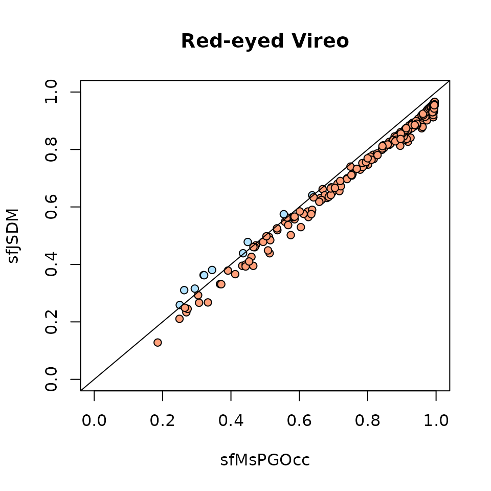
Not surprisingly, most estimates of occurrence probability are
smaller for the model that does not account for imperfect detection
(sfJSDM()). However, the differences here are not very
large for this species, which is exactly what we would expect for a
fairly common species. Let’s take a look at the results for a more rare
species (CAWA (Canda Warbler)).
curr.sp <- which(sp.ordered == 'CAWA')
# Color the points blue if sfJSDM > sfMsPGOcc, red otherwise
my.col <- ifelse(psi.mean.sfMsPGOcc[curr.sp, ] > psi.mean.sfJSDM[curr.sp, ],
         'lightsalmon', 'lightskyblue1')
plot(psi.mean.sfMsPGOcc[curr.sp, ], psi.mean.sfJSDM[curr.sp, ], pch = 21,
     bg = my.col, xlab = 'sfMsPGOcc', ylab = 'sfJSDM', main = 'Canada Warbler',
     ylim = c(0, 1), xlim = c(0, 1))
abline(0, 1)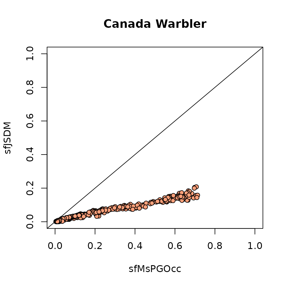
Here we see a clear discrepancy between the occurrence probability estimates from models that do and do not account for imperfect detection.
Prediction
We can use the predict() function to generate new
predictions of “occurrence” probability values given a set of covariates
and spatial locations. Note that these predictions are estimates of a
confounded probability of occurrence and detection (hence the quotations
around occurrence throughout this section). This code looks analogous to
what we saw with sfMsPGOcc().
# Not run (note this takes a large amount of memory to run).
data(hbefElev)
str(hbefElev)
elev.pred <- (hbefElev$val - mean(hbef.ordered$occ.covs[, 1])) / sd(hbef.ordered$occ.covs[, 1])
# Order: intercept, elevation (linear), elevation (quadratic)
X.0 <- cbind(1, elev.pred, elev.pred^2)
# Spatial coordinates
coords.0 <- as.matrix(hbefElev[, c('Easting', 'Northing')])
# Approximate run time: 30 sec
out.pred <- predict(out.sfJSDM, X.0, coords.0)
Latent factor joint species distribution models
The spOccupancy function lfJSDM() fits a
latent factor joint species distribution model. This model is analogous
to the latent factor multi-species occupancy model, except it does not
account for imperfect detection. Alternatively, the model can be viewed
as a non-spatial alternative to sfJSDM(). Just as we saw
with lfMsPGOcc(), we will account for species correlations
using a latent factor model, where the latent factors are assumed to
arise from independent standard normal distributions.
Basic model description
The latent factor joint species distribution model is identical to
the spatial factor joint species distribution model fit by
sfJSDM(), except now the latent factors do not have spatial
structure and are modeled using independent standard normal
distributions. See previous model descriptions for the spatial factor
joint species distribution model as well as the latent factor
multi-species occupancy model for additional details.
Fitting latent factor joint species distribution models with
lfJSDM
The function lfJSDM() fits latent factor joint species
distribution models using Pólya-Gamma data augmentation.
lfJSDM() has the following arguments.
lfJSDM(formula, data, inits, priors, n.factors,
       n.samples, n.omp.threads = 1, verbose = TRUE, n.report = 100,
       n.burn = round(.10 * n.samples), n.thin = 1, n.chains = 1,
       k.fold, k.fold.threads = 1, k.fold.seed, k.fold.only = FALSE, ...)
There are no new arguments in lfJSDM() that we have not
seen before in previous factor model functions. Notice that like
sfJSDM(), there is only a single formula since
we do not explicitly separate imperfect detection from latent
occurrence. Similar to sfJSDM(), the data list
should consist of the collapsed detection-nondetection data matrix
(y), the covariates (covs), and the spatial
coordinates (coords). We can use the same data list we
constructed previously for sfJSDM(), and we remind
ourselves of it’s structure below.
str(jsdm.list)List of 3
$ y : num [1:12, 1:373] 1 0 0 0 0 1 1 0 0 0 ...
..- attr(*, "dimnames")=List of 2
.. ..$ : chr [1:12] "OVEN" "BLPW" "AMRE" "BAWW" ...
.. ..$ : chr [1:373] "1" "2" "3" "4" ...
$ covs : num [1:373, 1] 475 494 546 587 588 ...
..- attr(*, "dimnames")=List of 2
.. ..$ : NULL
.. ..$ : chr "Elevation"
$ coords: num [1:373, 1:2] 280000 280000 280000 280001 280000 ...
..- attr(*, "dimnames")=List of 2
.. ..$ : chr [1:373] "1" "2" "3" "4" ...
.. ..$ : chr [1:2] "X" "Y"Specifying covariates in lfJSDM() is exactly analogous
to what we saw with sfJSDM(). Again, note that we can
include random intercepts in formula using lme4 syntax
(Bates et al. 2015). As we have done
before, we will use a single latent factor.
The remaining arguments are all identical to the arguments we saw in
lfMsPGOcc() when fitting a latent factor multi-species
occupancy model. See the section on “Fitting models with
lfMsPGOcc()” for specific details on these arguments. Note
that for the initial values and priors, we only need to specify these
values for the “occurrence” values since there is no detection
sub-model. Just like with sfJSDM(), we do not need to
specify initial values for the latent occurrence values \(z\) (since we assume perfect
detection).
# Initial values ----------------------
# Number of species
N <- nrow(jsdm.list$y)
# Initiate all lambda initial values to 0.
lambda.inits <- matrix(0, N, n.factors)
# Set diagonal elements to 1
diag(lambda.inits) <- 1
# Set lower triangular elements to random values from a standard normal dist
lambda.inits[lower.tri(lambda.inits)] <- rnorm(sum(lower.tri(lambda.inits)))
# Create list of initial values.
inits <- list(beta.comm = 0,
              beta = 0,
              tau.sq.beta = 1,
              lambda = lambda.inits)
# Priors ------------------------------
priors <- list(beta.comm.normal = list(mean = 0, var = 2.72),
               tau.sq.beta.ig = list(a = 0.1, b = 0.1))
# Additional arguments ----------------
n.samples <- 5000
n.burn <- 3000
n.thin <- 2
n.chains <- 3
n.report <- 1000
With all the arguments set for lfJSDM(), we are now
ready to run the model. We run the model for 5000 MCMC samples,
eliminating the first 3000 as burn-in and thinning by every 2
samples.
# Approx run time: 32 seconds
out.lfJSDM <- lfJSDM(formula = jsdm.formula,
                     data = jsdm.list,
                     inits = inits,
                     priors = priors,
                     n.factors = n.factors,
                     n.samples = n.samples,
                     n.report = n.report,
                     n.burn = n.burn,
                     n.thin = n.thin,
                     n.chains = n.chains)
----------------------------------------
Preparing to run the model
----------------------------------------
----------------------------------------
Model description
----------------------------------------
Latent Factor JSDM with Polya-Gamma latent
variable fit with 373 sites and 12 species.
Samples per Chain: 5000
Burn-in: 3000
Thinning Rate: 2
Number of Chains: 3
Total Posterior Samples: 3000
Using 1 latent factors.
Source compiled with OpenMP support and model fit using 1 thread(s).
----------------------------------------
Chain 1
----------------------------------------
Sampling ...
Sampled: 1000 of 5000, 20.00%
-------------------------------------------------
Sampled: 2000 of 5000, 40.00%
-------------------------------------------------
Sampled: 3000 of 5000, 60.00%
-------------------------------------------------
Sampled: 4000 of 5000, 80.00%
-------------------------------------------------
Sampled: 5000 of 5000, 100.00%
----------------------------------------
Chain 2
----------------------------------------
Sampling ...
Sampled: 1000 of 5000, 20.00%
-------------------------------------------------
Sampled: 2000 of 5000, 40.00%
-------------------------------------------------
Sampled: 3000 of 5000, 60.00%
-------------------------------------------------
Sampled: 4000 of 5000, 80.00%
-------------------------------------------------
Sampled: 5000 of 5000, 100.00%
----------------------------------------
Chain 3
----------------------------------------
Sampling ...
Sampled: 1000 of 5000, 20.00%
-------------------------------------------------
Sampled: 2000 of 5000, 40.00%
-------------------------------------------------
Sampled: 3000 of 5000, 60.00%
-------------------------------------------------
Sampled: 4000 of 5000, 80.00%
-------------------------------------------------
Sampled: 5000 of 5000, 100.00%
# Quick summary of model results
summary(out.lfJSDM)
Call:
lfJSDM(formula = jsdm.formula, data = jsdm.list, inits = inits,
    priors = priors, n.factors = n.factors, n.samples = n.samples,
    n.report = n.report, n.burn = n.burn, n.thin = n.thin, n.chains = n.chains)

Samples per Chain: 5000
Burn-in: 3000
Thinning Rate: 2
Number of Chains: 3
Total Posterior Samples: 3000
Run Time (min): 0.279

----------------------------------------
    Community Level
----------------------------------------
Means (logit scale):
                         Mean     SD    2.5%     50%  97.5%   Rhat  ESS
(Intercept)           -0.7713 0.8272 -2.4010 -0.7886 0.9137 1.0003 3000
scale(Elevation)       0.4046 0.4010 -0.3853  0.4019 1.2564 1.0094 2043
I(scale(Elevation)^2) -0.2641 0.1748 -0.6111 -0.2658 0.1028 1.0057 1507

Variances (logit scale):
                         Mean     SD   2.5%    50%   97.5%   Rhat  ESS
(Intercept)           10.7575 5.5869 4.3953 9.4254 25.6433 1.0024 2309
scale(Elevation)       1.9643 1.2923 0.6758 1.6663  4.8660 1.0053  956
I(scale(Elevation)^2)  0.3048 0.2246 0.0799 0.2453  0.8660 1.0021 1109

----------------------------------------
    Species Level
----------------------------------------
Estimates (logit scale):
                              Mean     SD    2.5%     50%   97.5%   Rhat  ESS
(Intercept)-OVEN            1.9950 0.2147  1.5990  1.9910  2.4336 1.0006 1843
(Intercept)-BLPW           -4.9667 0.6432 -6.3102 -4.9089 -3.8555 1.0160  245
(Intercept)-AMRE           -4.5734 0.6545 -6.0151 -4.5278 -3.4240 1.1270  314
(Intercept)-BAWW           -1.6119 0.2031 -2.0271 -1.6066 -1.2260 1.0018 1729
(Intercept)-BHVI           -2.0002 0.2651 -2.5629 -1.9835 -1.5280 1.0290  487
(Intercept)-BLBW            1.1663 0.1554  0.8752  1.1615  1.4734 1.0005 3000
(Intercept)-BTBW            3.2189 0.3777  2.5529  3.1948  4.0280 1.0169  417
(Intercept)-BTNW            1.9697 0.2249  1.5759  1.9669  2.4294 1.0016  982
(Intercept)-CAWA           -3.1234 0.3539 -3.8594 -3.0998 -2.4832 1.0056  601
(Intercept)-MAWA           -2.6962 0.3754 -3.4987 -2.6692 -2.0437 1.0536  318
(Intercept)-NAWA           -4.0448 0.5167 -5.2063 -3.9944 -3.1645 1.0060  308
(Intercept)-REVI            2.4093 0.2546  1.9520  2.3965  2.9677 1.0073 1113
scale(Elevation)-OVEN      -1.5047 0.1882 -1.8912 -1.4981 -1.1423 1.0030 1328
scale(Elevation)-BLPW       2.7798 0.6575  1.6907  2.6860  4.2548 1.0116  133
scale(Elevation)-AMRE       0.6548 0.6659 -0.5097  0.5940  2.1124 1.0108  207
scale(Elevation)-BAWW      -0.0672 0.2457 -0.5604 -0.0596  0.4174 1.0008 1165
scale(Elevation)-BHVI       0.1502 0.1596 -0.1517  0.1505  0.4677 0.9999 1693
scale(Elevation)-BLBW      -0.1997 0.1117 -0.4274 -0.1958  0.0183 1.0045 2734
scale(Elevation)-BTBW      -0.3232 0.1519 -0.6414 -0.3216 -0.0390 1.0035 1780
scale(Elevation)-BTNW       0.4893 0.1592  0.1819  0.4877  0.8050 1.0031 1939
scale(Elevation)-CAWA       1.5890 0.4728  0.7788  1.5481  2.5939 1.0375  271
scale(Elevation)-MAWA       1.6739 0.3084  1.1193  1.6539  2.3241 1.0335  437
scale(Elevation)-NAWA       1.1065 0.3440  0.5346  1.0764  1.8809 1.0142  437
scale(Elevation)-REVI      -1.1465 0.1851 -1.5263 -1.1407 -0.8043 1.0076 1151
I(scale(Elevation)^2)-OVEN -0.4861 0.1464 -0.7731 -0.4880 -0.2013 1.0026 1482
I(scale(Elevation)^2)-BLPW  0.5594 0.3531 -0.1521  0.5663  1.2200 1.0208  303
I(scale(Elevation)^2)-AMRE -0.6097 0.4362 -1.6139 -0.5760  0.1540 1.0039  347
I(scale(Elevation)^2)-BAWW -0.7066 0.2246 -1.1990 -0.6896 -0.3187 1.0102  751
I(scale(Elevation)^2)-BHVI  0.0524 0.1319 -0.2124  0.0531  0.3015 1.0145 1511
I(scale(Elevation)^2)-BLBW -0.3132 0.0928 -0.5013 -0.3129 -0.1392 1.0018 3306
I(scale(Elevation)^2)-BTBW -0.9184 0.1470 -1.2238 -0.9138 -0.6449 1.0048  748
I(scale(Elevation)^2)-BTNW -0.1301 0.1161 -0.3569 -0.1286  0.0968 1.0017 2200
I(scale(Elevation)^2)-CAWA -0.4975 0.2975 -1.1127 -0.4855  0.0377 1.0325  406
I(scale(Elevation)^2)-MAWA  0.0498 0.2080 -0.3669  0.0486  0.4433 1.0044  839
I(scale(Elevation)^2)-NAWA  0.1964 0.2326 -0.2925  0.2008  0.6294 1.0127  669
I(scale(Elevation)^2)-REVI -0.3818 0.1434 -0.6612 -0.3833 -0.0886 1.0088 1478
Not surprisingly, lfJSDM() is the fastest of the four
models we have fit to the Hubbard Brook data. This makes sense since it
only accounts for one (residual species correlations) of the three
complexities and ignores the other two (imperfect detection and spatial
autocorrelation). Note that we also see nice converging and mixing of
all model parameters. This is a constant battle we fight with fitting
Bayesian models. Generally, the more complex a model is, the longer it
takes to run to reach convergence. For more simple models like the
latent factor joint species distribution model, models usually run quite
fast and we often will see adequate convergence and mixing without
having to run too many MCMC samples.
Model selection using WAIC
We compute the WAIC for latent factor JSDMs using the
waicOcc() function, and we compare this value to the WAIC
for the spatial factor JSDM we fit with sfJSDM().
waicOcc(out.lfJSDM) elpd pD WAIC
-1271.5117 180.8208 2904.6649
waicOcc(out.sfJSDM) elpd pD WAIC
-1279.1249 142.2271 2842.7040 The WAIC value for the spatial factor JSDM is smaller than that of
the latnet factor JSDM, indicating that accounting for spatial
autocorrelation improves model fit. As we noted for
sfJSDM(), we cannot directly compare the WAIC value from a
latent factor JSDM to those obtained from lfMsPGOcc() or
sfMsPGOcc() since they do not use the same data. As with
all factor model functions, we can additionaly use k-fold
cross-validation to assess out-of-sample predictive performance. See the
main spOccupancy vignette for examples of
cross-validation using spOccupancy model functions.
Prediction
We can use the predict() function to generate new
predictions of “occurrence” probability values given a set of covariates
and spatial locations. Again, note that these predictions are estimates
of a confounded probability of occurrence and detection. This code is
analogous to what we saw with lfMsPGOcc().
# Not run (note this takes a large amount of memory to run).
data(hbefElev)
elev.pred <- (hbefElev$val - mean(hbef2015$occ.covs[, 1])) / sd(hbef2015$occ.covs[, 1])
# Order: intercept, elevation (linear), elevation (quadratic)
X.0 <- cbind(1, elev.pred, elev.pred^2)
# Spatial coordinates
coords.0 <- as.matrix(hbefElev[, c('Easting', 'Northing')])
# Approximate run time: 30 sec
out.pred <- predict(out.lfJSDM, X.0, coords.0)
str(out.pred)
# Species richness samples
rich.pred <- apply(out.pred$z.0.samples, c(1, 3), sum)
plot.dat <- data.frame(x = hbefElev$Easting,
                       y = hbefElev$Northing,
                       rich.mean = apply(rich.pred, 2, mean),
                       rich.sd = apply(rich.pred, 2, sd))
# Plot species richness of the foliage-gleaning bird community
# across the Hubbard Brook Experimental Forest
dat.stars <- st_as_stars(plot.dat, dims = c('x', 'y'))
ggplot() +
  geom_stars(data = dat.stars, aes(x = x, y = y, fill = rich.mean)) +
  scale_fill_viridis_c(na.value = 'transparent') +
  labs(x = 'Easting', y = 'Northing', fill = '',
       title = 'Mean Species Richness') +
  theme_bw()