Exploring model identifiability with a stress-testing framework
Sara Stoudt
October 26, 2023
Source:vignettes/identifiability.Rmd
identifiability.RmdOverview of identifiability and stress-testing framework
We rarely believe that our model is a perfect representation of a natural phenomenon; nature is complicated after all. Because of this, we need to make sure that our model is robust to mis-specification. Namely, we want to make sure that our ability to uniquely identify parameters of interest does not just come from a convenient choice of model structure. Formally, this is a question of identifiability. To explore whether our scenario has weak or strong identifiability we can go through the following steps:
- Simulate data from a data-generating process that does not match the model fitting process.
- Fit mis-specified models, allowing for more flexibility (within the mis-specified model family) using a spline basis of covariates in the model fit.
- Explore performance across a variety of sample sizes looking for a break down in estimation.
For more information on this stress-testing framework, along with a more thorough discussion on the different types of identifiability in statistical models, see Stoudt, de Valpine, and Fithian (2023). This type of framework is particularly relevant for assessing identifiability in occupancy models with limited data, such as when trying to separately estimate occupancy and detection in so-called “single-visit” models, where there is only one visit to each site in the data set (Lele, Moreno, and Bayne 2012). Here we provide a simple example of a stress testing framework in which we compare identifiability of occurrence probability in single-visit occupancy models compared to double-visit occupancy models (where each site is visited two times).
library(spOccupancy)
library(splines) # For creating spline basis of covariates
Simulate data
To diagnose a weak form of identifiability, we need to see how a model performs on data from a data-generating process that does not match the model. We will want to generate these data under a variety of sample sizes including sizes larger than we expect to see in practice.
An updated version of the simTOcc function introduced in
v0.6.0
allows us to simulate data from two different classes of data-generating
processes:
- a scaled logistic where occurrence and detection probabilities still are related to covariates via a logit link but the occurrence probabilities level off at a value less than one, and
- a linear specification where occurrence and detection probabilities are linearly related to covariates (while the values respect the probability range within the range of covariate values observed).
In this vignette, we will show the most extreme mis-specification
(scaled logistic with mis.spec.type = 'scale' where the
scale.param argument represents the scaling parameter for
the occurrence probabilities) in the largest data case. Here the choice
of 0.8 means that the maximum occurrence probability is 0.8 rather than
1. See Stoudt, de Valpine, and Fithian
(2023) for more details on this form of mis-specification.
# Number of simulated data sets for each scenario
n.sims <- 25
# Set seed to keep results consistent
set.seed(12798)
# Spatial locations
J.x <- c(10, 32, 100)
J.y <- c(10, 32, 100)
J <- J.x * J.y
# Three different amounts of spatial locations

# For single visit scenarios, we double the number of sites
# compared to single visits so that the double visit data
# are "richer" data, not just more data. Not necessary, but
# can help make the case more convincing.
J2 <- 2 * J.x * J.y

# Number of years
n.time <- 1

# Occurrence coefficient --------------
# Intercept and a single covariate
beta <- c(-1, 1)
p.occ <- length(beta)

# Detection coefficient ---------------
# Intercept and a single covariate
alpha <- c(-2, 0.5)

# No spatial or temporal autocorrelation
sp <- FALSE
trend <- FALSE

# Set up vectors to hold data sets
sv_dat_small <- dv_dat_small <- vector("list", n.sims)
sv_dat_medium <- dv_dat_medium <- vector("list", n.sims)
sv_dat_large <- dv_dat_large <- vector("list", n.sims)

# Simulate multiple datasets under each scenario
for (i in 1:n.sims) {
  # Small, single-visit
  sv_dat_small[[i]] <- simTOcc(
    J.x = 2 * J.x[1], J.y = J.y[1], n.time = rep(n.time, J2[1]),
    beta = beta, alpha = alpha,
    n.rep = matrix(1, J2[1], n.time), sp = sp,
    trend = trend, scale.param = 0.5, mis.spec.type = "scale"
  )
  # Small, double-visit
  dv_dat_small[[i]] <- simTOcc(
    J.x = J.x[1], J.y = J.y[1], n.time = rep(n.time, J[1]),
    beta = beta, alpha = alpha,
    n.rep = matrix(2, J[1], n.time), sp = sp,
    trend = trend, scale.param = 0.5, mis.spec.type = "scale"
  )

  # Medum, single-visit
  sv_dat_medium[[i]] <- simTOcc(
    J.x = 2 * J.x[2], J.y = J.y[2], n.time = rep(n.time, J2[2]),
    beta = beta, alpha = alpha,
    n.rep = matrix(1, J2[2], n.time), sp = sp,
    trend = trend, scale.param = 0.5, mis.spec.type = "scale"
  )
  # Medium, double-visit
  dv_dat_medium[[i]] <- simTOcc(
    J.x = J.x[2], J.y = J.y[2], n.time = rep(n.time, J[2]),
    beta = beta, alpha = alpha,
    n.rep = matrix(2, J[2], n.time), sp = sp,
    trend = trend, scale.param = 0.5, mis.spec.type = "scale"
  )

  # Large, single visit
  # Here we'll focus on the large case for the sake of brevity, but
  # you will want to see the build up if applying this to your own work
  sv_dat_large[[i]] <- simTOcc(
    J.x = 2 * J.x[3], J.y = J.y[3], n.time = rep(n.time, J2[3]),
    beta = beta, alpha = alpha,
    n.rep = matrix(1, J2[3], n.time), sp = sp,
    trend = trend, scale.param = 0.5, mis.spec.type = "scale"
  )
  dv_dat_large[[i]] <- simTOcc(
    J.x = J.x[3], J.y = J.y[3], n.time = rep(n.time, J[3]),
    beta = beta, alpha = alpha,
    n.rep = matrix(2, J[3], n.time), sp = sp,
    trend = trend, scale.param = 0.5, mis.spec.type = "scale"
  )
}
Now we have 25 small, medium, and large datasets for both single and
double visit cases. The typical spOccupancy model fit will
be mis-specified for data that come from this data-generating
process.
Create basis splines for a flexible model fit
Let’s fit a flexible model to one of the large data scenarios. This
will show that even with an extreme amount of data, a lack of
strong identifiability cannot be overcome without richer data
(a double visit at each site). First we need to create a spline basis
from the covariates provided by simTOcc, and then we need
to reformat the data so that it is appropriate for the required inputs
of the PGOcc function. The spline basis helps the model be
more flexible. We want to approximate a nonparametric relationship
between the response and the covariate to give the mis-specified model
more freedom to recover the truth as compared to the specific parametric
model. If a flexible model with enough data can recover the truth, that
provides evidence that the model is fit for purpose even when formally
mis-specified. We can trust its estimates are not chosen by fiat
(determined by an arbitrary choice of model) but rather reflect some
property of the underlying ecology.
# Work with large, single-visit data for now.
dat <- sv_dat_large[[1]]

# Site x Replicate data set
y <- dat$y
# Occurrence Covariates
X <- dat$X
# Detection Covariates
X.p <- dat$X.p

# Create a spline basis for each covariate --------------------------------
numKnots <- 7
m <- 1:numKnots
psiBound <- c(floor(min(X[, , 2])), ceiling(max(X[, , 2])))
pBound <- c(floor(min(X.p[, , , 2])), ceiling(max(X.p[, , , 2])))

X.sp_SV <- as.data.frame(bs(X[, , 2], knots = psiBound[1] + m * psiBound[2] / (numKnots + 1)))
X.p.sp_SV <- bs(X.p[, , , 2], knots = pBound[1] + m * pBound[2] / (numKnots + 1))

detectCovFormattedSV <- vector("list", numKnots + 3)
for (j in 1:(numKnots + 3)) {
  detectCovFormattedSV[[j]] <- X.p.sp_SV[, j]
}

names(X.sp_SV) <- paste("z", 1:(numKnots + 3), sep = "")
names(detectCovFormattedSV) <- paste("p", 1:(numKnots + 3), sep = "")


# Put data sets in spOccupancy format
formattedData_SV <- list(
  y = y, occ.covs = X.sp_SV,
  det.covs = detectCovFormattedSV
)
# Take a look
str(formattedData_SV)
List of 3
$ y : int [1:20000, 1, 1] 0 0 0 0 0 0 0 0 0 0 ...
$ occ.covs:'data.frame': 20000 obs. of 10 variables:
..$ z1 : num [1:20000] 0 0 0 0 0 0 0 0 0 0 ...
..$ z2 : num [1:20000] 0 0 0 0 0 0 0 0 0 0 ...
..$ z3 : num [1:20000] 0 0 0 0 0 0 0 0 0 0 ...
..$ z4 : num [1:20000] 0 0 0 0 0 0 0 0 0 0 ...
..$ z5 : num [1:20000] 0 0 0 0 0 ...
..$ z6 : num [1:20000] 0 0 0 0 0.132 ...
..$ z7 : num [1:20000] 0.232 0.673 0.408 0.398 0.811 ...
..$ z8 : num [1:20000] 0.4799 0.3075 0.4663 0.4697 0.0571 ...
..$ z9 : num [1:20000] 2.56e-01 2.00e-02 1.20e-01 1.26e-01 4.42e-06 ...
..$ z10: num [1:20000] 3.24e-02 2.35e-05 5.60e-03 6.28e-03 0.00 ...
$ det.covs:List of 10
..$ p1 : num [1:20000] 0 0 0 0 0 0 0 0 0 0 ...
..$ p2 : num [1:20000] 0 0 0 0 0 0 0 0 0 0 ...
..$ p3 : num [1:20000] 0 0 0 0 0 0 0 0 0 0 ...
..$ p4 : num [1:20000] 0 0 0 0 0 ...
..$ p5 : num [1:20000] 0 0 0 0.034 0 ...
..$ p6 : num [1:20000] 0 0.0157 0 0.5324 0 ...
..$ p7 : num [1:20000] 0.187 0.832 0.347 0.43 0.395 ...
..$ p8 : num [1:20000] 0.46134 0.15022 0.48224 0.00316 0.47024 ...
..$ p9 : num [1:20000] 0.30266 0.00163 0.15954 0 0.1279 ...
..$ p10: num [1:20000] 0.04948 0 0.01084 0 0.00654 ...We’re now set to run models using the PGOcc() function
in spOccupancy. We set up the necessary arguments for the
function below, and then run the model for the first simulated data
set.
occ.formula <- formula(paste("~", paste("z", 1:(numKnots + 3), sep = "", collapse = "+")))
det.formula <- formula(paste("~", paste("p", 1:(numKnots + 3), sep = "", collapse = "+")))

# MCMC criteria
n.samples <- 5000
n.burn <- 3000
n.thin <- 2
n.chains <- 3


# Priors
# Note that we don't scale the covariates, so we increase the variance of the priors to be larger,
# which differs from the default spOccupancy value of 2.72
prior.list <- list(
  beta.normal = list(mean = 0, var = 100),
  alpha.normal = list(mean = 0, var = 100)
)

# Initial values set to 0
initsSV <- list(
  alpha = rep(0, length(formattedData_SV$det.covs) + 1),
  beta = rep(0, ncol(formattedData_SV$occ.covs) + 1), z = as.vector(formattedData_SV$y)
)

# Fitting large datasets can take some time - this one takes about 3 minutes
out_sv <- PGOcc(
  occ.formula = occ.formula, det.formula = det.formula,
  data = formattedData_SV,
  inits = initsSV, n.samples = n.samples, priors = prior.list,
  n.omp.threads = 1, verbose = F, n.report = 1000,
  n.burn = n.burn, n.thin = n.thin, n.chains = n.chains
)

# Occurrence coefficient estimates
occur_est <- apply(out_sv$beta.samples, 2, mean)
# Detection coefficient estimates
detect_est <- apply(out_sv$alpha.samples, 2, mean)
Below we do the same thing, but now for the double visit scenario.
# Work with large, double-visit data
dat <- dv_dat_large[[1]]

# Site x Replicate
y <- dat$y[, , 1:2]
# Occurrence Covariates
X <- dat$X
# Detection Covariates
X.p <- dat$X.p

# Create a spline basis for each covariate
numKnots <- 7
m <- 1:numKnots
psiBound <- c(floor(min(X[, , 2])), ceiling(max(X[, , 2])))
pBound <- c(floor(min(X.p[, , , 2])), ceiling(max(X.p[, , , 2])))

X.sp <- as.data.frame(bs(X[, , 2], knots = psiBound[1] + m * psiBound[2] / (numKnots + 1)))
X.p.sp <- bs(X.p[, , , 2], knots = pBound[1] + m * pBound[2] / (numKnots + 1))

detectCovFormatted <- vector("list", numKnots + 3)
for (j in 1:(numKnots + 3)) {
  detectCovFormatted[[j]] <- X.p.sp[, j]
}

names(X.sp) <- paste("z", 1:(numKnots + 3), sep = "")
names(detectCovFormatted) <- paste("p", 1:(numKnots + 3), sep = "")

# Get data in spOccupancy format.
formattedData <- list(
  y = y, occ.covs = X.sp,
  det.covs = detectCovFormatted
)

occ.formula <- formula(paste("~", paste("z", 1:(numKnots + 3), sep = "", collapse = "+")))
det.formula <- formula(paste("~", paste("p", 1:(numKnots + 3), sep = "", collapse = "+")))

# MCMC criteria
n.samples <- 5000
n.burn <- 3000
n.thin <- 2
n.chains <- 3


# Priors, same as before
prior.list <- list(
  beta.normal = list(mean = 0, var = 100),
  alpha.normal = list(mean = 0, var = 100)
)

# Initial values
initsDV <- list(
  alpha = rep(0, length(formattedData$det.covs) + 1),
  beta = rep(0, ncol(formattedData$occ.covs) + 1), z = apply(formattedData$y, 1, max, na.rm = T)
)

# Run the model with PGOcc
out_dv <- PGOcc(
  occ.formula = occ.formula, det.formula = det.formula,
  data = formattedData,
  inits = initsDV, n.samples = n.samples, priors = prior.list,
  n.omp.threads = 1, verbose = F, n.report = 1000,
  n.burn = n.burn, n.thin = n.thin, n.chains = n.chains
)

# Occurrence regression coefficients
occur_estDV <- apply(out_dv$beta.samples, 2, mean)
# Detection regression coefficients
detect_estDV <- apply(out_dv$alpha.samples, 2, mean)
Examine results
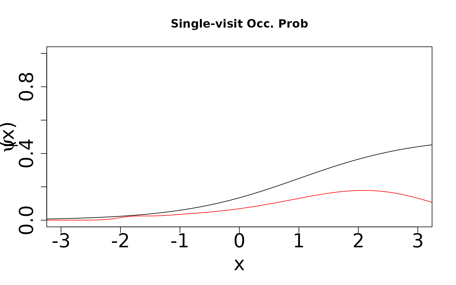
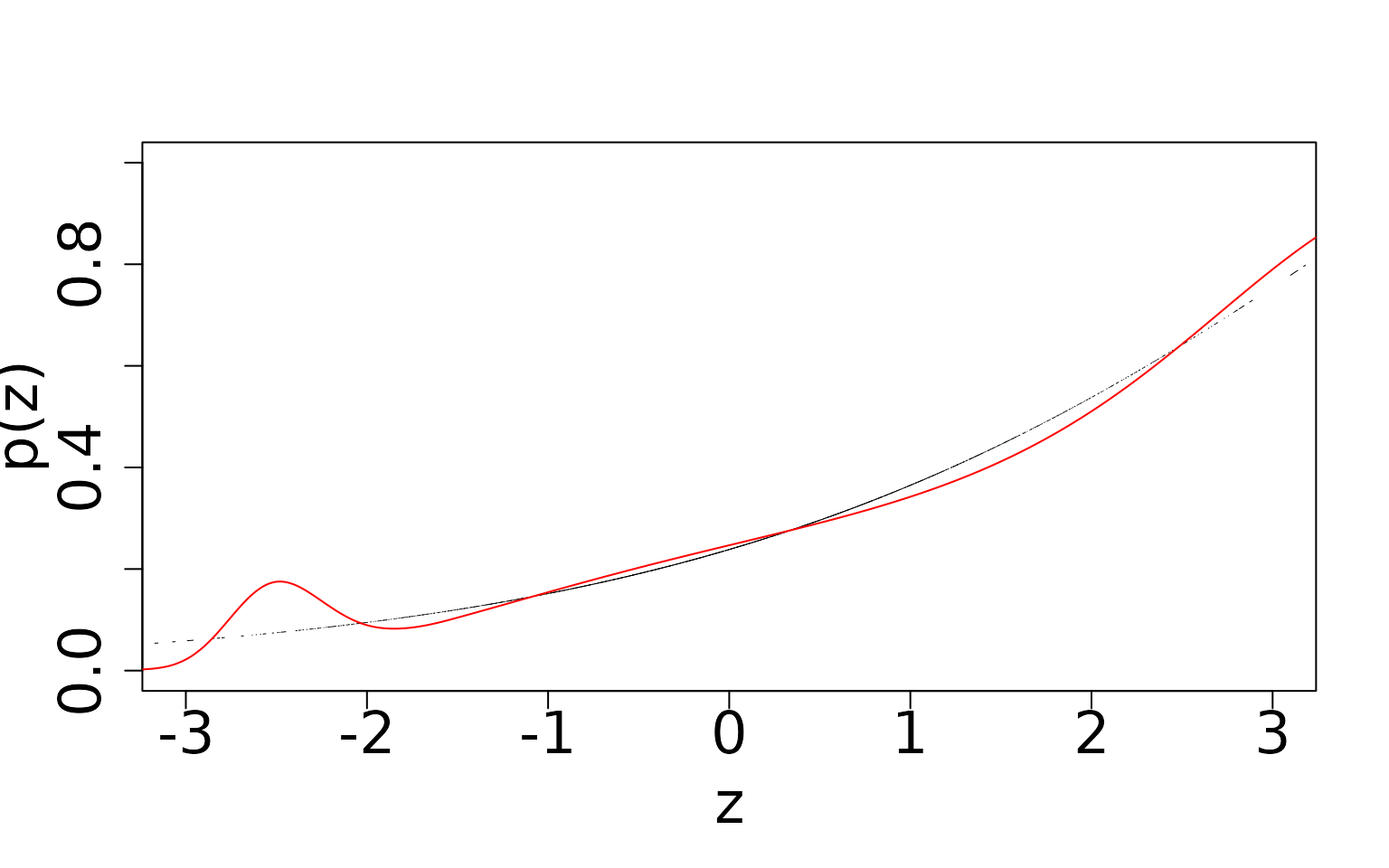
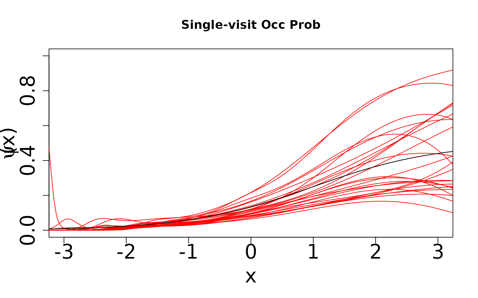
Now, because we know the truth, we can display the true values against the predicted values. We expect the single visit case to not estimate the true values because the data-generating process does not match the assumed modeling framework and this scenario is only weakly (parametrically) identifiable (Stoudt, de Valpine, and Fithian 2023). However, we expect the double visit case to estimate something close to the truth even though it is still mis-specified. This case is more strongly identifiable and hence should be robust to mis-specification. In the plots shown below, the black line is the true relationship and the red lines are our estimates.
dat <- sv_dat_large[[1]]
zData <- dat$X[, , 2]
psiData <- dat$psi[, 1]
idx <- order(zData)
thin <- 1:length(zData)
basisPsiSV <- X.sp_SV

# Plot the true values
plot((zData[idx])[thin], (psiData[idx])[thin], ylim = c(0, 1), type = "l",
     lwd = .5, xlim = c(-3, 3), xlab = "x", ylab = "",
     cex.axis = 2, cex.lab = 2, main = 'Single-visit Occ. Prob')

# Generate predicted occurrence probability values and plot
fitted.val <- exp(occur_est[[1]] +
  occur_est[[2]] * basisPsiSV[, 1] +
  occur_est[[3]] * basisPsiSV[, 2] +
  occur_est[[4]] * basisPsiSV[, 3] +
  occur_est[[5]] * basisPsiSV[, 4] +
  occur_est[[6]] * basisPsiSV[, 5] +
  occur_est[[7]] * basisPsiSV[, 6]
  + occur_est[[8]] * basisPsiSV[, 7]
  + occur_est[[9]] * basisPsiSV[, 8]
  + occur_est[[10]] * basisPsiSV[, 9]
  + occur_est[[11]] * basisPsiSV[, 10]) / (1 + exp(occur_est[[1]] +
  occur_est[[2]] * basisPsiSV[, 1] +
  occur_est[[3]] * basisPsiSV[, 2] +
  occur_est[[4]] * basisPsiSV[, 3] +
  occur_est[[5]] * basisPsiSV[, 4] +
  occur_est[[6]] * basisPsiSV[, 5] +
  occur_est[[7]] * basisPsiSV[, 6]
  + occur_est[[8]] * basisPsiSV[, 7]
  + occur_est[[9]] * basisPsiSV[, 8]
  + occur_est[[10]] * basisPsiSV[, 9]
  + occur_est[[11]] * basisPsiSV[, 10]))
lines((zData[idx]), (fitted.val[idx]), col = "red", cex = .5)
lines(zData[idx][thin], psiData[idx][thin])
mtext(
  text = expression(paste(psi, "(x)")),
  side = 2,
  line = 2.5, cex = 2
)
Now we generate the same figure, but for detection probability
mData <- dat$X.p[, , , 2]
pData <- dat$p[, , 1]
idx <- order(mData)
thin <- 1:length(mData)
basisPSV <- X.p.sp_SV
plot((mData[idx])[thin], (pData[idx])[thin], ylim = c(0, 1), type = "l",
lwd = .5, xlim = c(-3, 3), xlab = "z", ylab = "", cex.axis = 2,
cex.lab = 2, main = 'Single-visit Det. Prob')
# Generate predicted detection probability values and plot
fitted.val <- exp(detect_est[[1]] +
detect_est[[2]] * basisPSV[, 1] +
detect_est[[3]] * basisPSV[, 2] +
detect_est[[4]] * basisPSV[, 3] +
detect_est[[5]] * basisPSV[, 4] +
detect_est[[6]] * basisPSV[, 5] +
detect_est[[7]] * basisPSV[, 6]
+ detect_est[[8]] * basisPSV[, 7]
+ detect_est[[9]] * basisPSV[, 8]
+ detect_est[[10]] * basisPSV[, 9]
+ detect_est[[11]] * basisPSV[, 10]) / (1 + exp(detect_est[[1]] +
detect_est[[2]] * basisPSV[, 1] +
detect_est[[3]] * basisPSV[, 2] +
detect_est[[4]] * basisPSV[, 3] +
detect_est[[5]] * basisPSV[, 4] +
detect_est[[6]] * basisPSV[, 5] +
detect_est[[7]] * basisPSV[, 6]
+ detect_est[[8]] * basisPSV[, 7]
+ detect_est[[9]] * basisPSV[, 8]
+ detect_est[[10]] * basisPSV[, 9]
+ detect_est[[11]] * basisPSV[, 10]))
lines((mData[idx])[thin], (fitted.val[idx])[thin], col = "red", cex = .5)
mtext(
text = expression(paste(p, "(z)")),
side = 2,
line = 2.5, cex = 2
)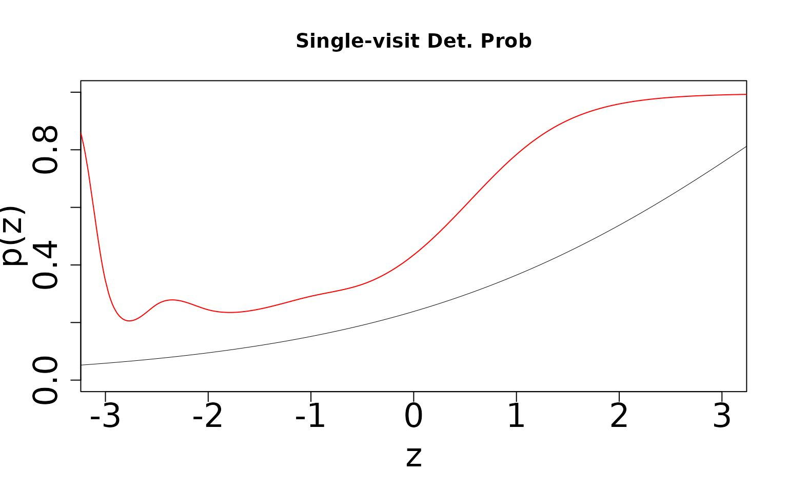 Note that we underestimate occurrence and overestimate detection. The
product of the two is identifiable, but teasing them apart requires two
visits. We can see this by generating the same two figures for the
double-visit simulation.
Note that we underestimate occurrence and overestimate detection. The
product of the two is identifiable, but teasing them apart requires two
visits. We can see this by generating the same two figures for the
double-visit simulation.
# Occurrence probability, double-visit
dat <- dv_dat_large[[1]]
zData <- dat$X[, , 2]
psiData <- dat$psi[, 1]
idx <- order(zData)
thin <- 1:length(zData)
basisPsi <- X.sp

# Plot the truth
plot((zData[idx])[thin], (psiData[idx])[thin], ylim = c(0, 1), type = "l",
     lwd = .5, xlim = c(-3, 3), xlab = "x", ylab = "",
     cex.axis = 2, cex.lab = 2, main = 'Double-visit Occ Prob')

# Generate predicted occurrence probability and plot
fitted.val <- exp(occur_estDV[[1]] +
  occur_estDV[[2]] * basisPsi[, 1] +
  occur_estDV[[3]] * basisPsi[, 2] +
  occur_estDV[[4]] * basisPsi[, 3] +
  occur_estDV[[5]] * basisPsi[, 4] +
  occur_estDV[[6]] * basisPsi[, 5] +
  occur_estDV[[7]] * basisPsi[, 6]
  + occur_estDV[[8]] * basisPsi[, 7]
  + occur_estDV[[9]] * basisPsi[, 8]
  + occur_estDV[[10]] * basisPsi[, 9]
  + occur_estDV[[11]] * basisPsi[, 10]) / (1 + exp(occur_estDV[[1]] +
  occur_estDV[[2]] * basisPsi[, 1] +
  occur_estDV[[3]] * basisPsi[, 2] +
  occur_estDV[[4]] * basisPsi[, 3] +
  occur_estDV[[5]] * basisPsi[, 4] +
  occur_estDV[[6]] * basisPsi[, 5] +
  occur_estDV[[7]] * basisPsi[, 6]
  + occur_estDV[[8]] * basisPsi[, 7]
  + occur_estDV[[9]] * basisPsi[, 8]
  + occur_estDV[[10]] * basisPsi[, 9]
  + occur_estDV[[11]] * basisPsi[, 10]))

lines((zData[idx]), (fitted.val[idx]), col = "red", cex = .5)

lines(sort(zData[[1]][thin]), sort(psiData[[1]][thin]))

mtext(
  text = expression(paste(psi, "(x)")),
  side = 2,
  line = 2.5, cex = 2
)
# Detection probability, double-visit
mData <- dat$X.p[, , , 2]
pData <- dat$p[, , 1]
idx <- order(mData)
thin <- 1:length(mData)
basisP <- X.p.sp
plot((mData[idx])[thin], (pData[idx])[thin], ylim = c(0, 1), type = "l", lwd = .5, xlim = c(-3, 3), xlab = "z", ylab = "", cex.axis = 2, cex.lab = 2) ## truth

## predicted value

fitted.val <- exp(detect_estDV[[1]] +
  detect_estDV[[2]] * basisP[, 1] +
  detect_estDV[[3]] * basisP[, 2] +
  detect_estDV[[4]] * basisP[, 3] +
  detect_estDV[[5]] * basisP[, 4] +
  detect_estDV[[6]] * basisP[, 5] +
  detect_estDV[[7]] * basisP[, 6]
  + detect_estDV[[8]] * basisP[, 7]
  + detect_estDV[[9]] * basisP[, 8]
  + detect_estDV[[10]] * basisP[, 9]
  + detect_estDV[[11]] * basisP[, 10]) / (1 + exp(detect_estDV[[1]] +
  detect_estDV[[2]] * basisP[, 1] +
  detect_estDV[[3]] * basisP[, 2] +
  detect_estDV[[4]] * basisP[, 3] +
  detect_estDV[[5]] * basisP[, 4] +
  detect_estDV[[6]] * basisP[, 5] +
  detect_estDV[[7]] * basisP[, 6]
  + detect_estDV[[8]] * basisP[, 7]
  + detect_estDV[[9]] * basisP[, 8]
  + detect_estDV[[10]] * basisP[, 9]
  + detect_estDV[[11]] * basisP[, 10]))


lines((mData[idx])[thin], (fitted.val[idx])[thin], col = "red", cex = .5)
mtext(
  text = expression(paste(p, "(z)")),
  side = 2,
  line = 2.5, cex = 2
)
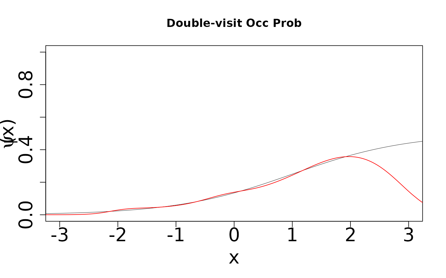
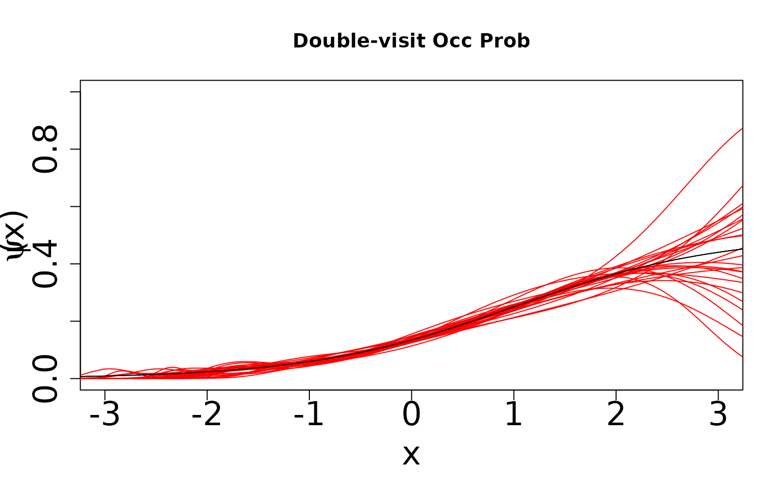
Even though this model is formally mis-specified, we can see that the
richer data (the extra visit) allows us to still estimate occurrence and
detection probabilities well. This model is robust to this form of of
model mis-specification. You may be wondering why the estimated curves
in the double-visit simulation deviate a bit from the true curve at the
extreme values of the covariate. This is related to how the covariates
were simulated. In particular, the simulation functions in
spOccupancy generate covariates as standard normal random
variables, which means values on the extremes will be very rare. In
these portions of the curve, the spline models are only informed by a
small number of data points, and hence any sort of sampling variability
that can arise in a single simulated data set can result in some
deviations from the true curve. When performing multiple simulations, we
should see that any given simulation may show some slight variation at
the boundaries of the covariate space, but that on average across
simulations occupancy/detection probability are estimated close to the
true values. If we simulate the covariates in a different manner, e.g.,
using a uniform distribution, this pattern disappears. We leave that to
you to explore on your own time if it is of interest.
Multiple scenarios
To ensure that this is not a fluke, we can look across multiple scenarios. This will take a bit of time to run for larger datasets, so we’ll just show the code and results.
occur_est <- detect_est <- X.sp_SV <- X.p.sp_SV <- vector("list", length(sv_dat_large))
# Prep data and run the models --------------------------------------------
for (i in 1:length(sv_dat_large)) {
  print(paste0("Currently on simulation ", i, " out of ", length(sv_dat_large)))
  dat <- sv_dat_large[[i]]

  # Site x Replicate
  y <- dat$y
  # Occurrence Covariates
  X <- dat$X
  # Detection Covariates
  X.p <- dat$X.p

  # Create a spline basis for each covariate
  numKnots <- 7
  m <- 1:numKnots
  psiBound <- c(floor(min(X[, , 2])), ceiling(max(X[, , 2])))
  pBound <- c(floor(min(X.p[, , , 2])), ceiling(max(X.p[, , , 2])))

  X.sp_SV[[i]] <- as.data.frame(bs(X[, , 2], knots = psiBound[1] + m * psiBound[2] / (numKnots + 1)))
  X.p.sp_SV[[i]] <- bs(X.p[, , , 2], knots = pBound[1] + m * pBound[2] / (numKnots + 1))

  detectCovFormattedSV <- vector("list", numKnots + 3)
  for (j in 1:(numKnots + 3)) {
    detectCovFormattedSV[[j]] <- X.p.sp_SV[[i]][, j]
  }

  names(X.sp_SV[[i]]) <- paste("z", 1:(numKnots + 3), sep = "")
  names(detectCovFormattedSV) <- paste("p", 1:(numKnots + 3), sep = "")


  formattedData_SV <- list(
    y = y, occ.covs = X.sp_SV[[i]],
    det.covs = detectCovFormattedSV
  )


  occ.formula <- formula(paste("~", paste("z", 1:(numKnots + 3), sep = "", collapse = "+")))
  det.formula <- formula(paste("~", paste("p", 1:(numKnots + 3), sep = "", collapse = "+")))


  n.samples <- 5000
  n.burn <- 3000
  n.thin <- 2
  n.chains <- 3


  # Priors
  prior.list <- list(
    beta.normal = list(mean = 0, var = 100),
    alpha.normal = list(mean = 0, var = 100)
  )

  initsSV <- list(
    alpha = rep(0, length(formattedData_SV$det.covs) + 1),
    beta = rep(0, ncol(formattedData_SV$occ.covs) + 1), z = as.vector(formattedData_SV$y)
  )

  out_sv <- PGOcc(
    occ.formula = occ.formula, det.formula = det.formula,
    data = formattedData_SV,
    inits = initsSV, n.samples = n.samples, priors = prior.list,
    n.omp.threads = 1, verbose = F, n.report = 1000,
    n.burn = n.burn, n.thin = n.thin, n.chains = n.chains
  )

  occur_est[[i]] <- apply(out_sv$beta.samples, 2, mean)
  detect_est[[i]] <- apply(out_sv$alpha.samples, 2, mean)
}
dat <- sv_dat_large[[1]]
zData <- dat$X[, , 2]
psiData <- dat$psi[, 1]
idx <- order(zData)
thin <- 1:length(zData)
basisPsiSV <- X.sp_SV[[1]]

plot((zData[idx])[thin], (psiData[idx])[thin], ylim = c(0, 1), type = "l",
     lwd = .5, xlim = c(-3, 3), xlab = "x", ylab = "",
     cex.axis = 2, cex.lab = 2, main = 'Single-visit Occ Prob')
for (i in 2:length(occur_est)) {
  dat <- sv_dat_large[[i]]
  zData <- dat$X[, , 2]
  psiData <- dat$psi[, 1]
  idx <- order(zData)
  thin <- 1:length(zData)
  basisPsiSV <- X.sp_SV[[i]]
  idx <- order(zData)
  lines((zData[idx])[thin], (psiData[idx])[thin], lwd = .5)
}

for (i in 1:length(sv_dat_large)) {
  dat <- sv_dat_large[[i]]
  zData <- dat$X[, , 2]
  psiData <- dat$psi[, 1]
  idx <- order(zData)
  thin <- 1:length(zData)
  basisPsiSV <- X.sp_SV[[i]]
  fitted.val <- exp(occur_est[[i]][[1]] +
    occur_est[[i]][[2]] * basisPsiSV[, 1] +
    occur_est[[i]][[3]] * basisPsiSV[, 2] +
    occur_est[[i]][[4]] * basisPsiSV[, 3] +
    occur_est[[i]][[5]] * basisPsiSV[, 4] +
    occur_est[[i]][[6]] * basisPsiSV[, 5] +
    occur_est[[i]][[7]] * basisPsiSV[, 6]
    + occur_est[[i]][[8]] * basisPsiSV[, 7]
    + occur_est[[i]][[9]] * basisPsiSV[, 8]
    + occur_est[[i]][[10]] * basisPsiSV[, 9]
    + occur_est[[i]][[11]] * basisPsiSV[, 10]) / (1 + exp(occur_est[[i]][[1]] +
    occur_est[[i]][[2]] * basisPsiSV[, 1] +
    occur_est[[i]][[3]] * basisPsiSV[, 2] +
    occur_est[[i]][[4]] * basisPsiSV[, 3] +
    occur_est[[i]][[5]] * basisPsiSV[, 4] +
    occur_est[[i]][[6]] * basisPsiSV[, 5] +
    occur_est[[i]][[7]] * basisPsiSV[, 6]
    + occur_est[[i]][[8]] * basisPsiSV[, 7]
    + occur_est[[i]][[9]] * basisPsiSV[, 8]
    + occur_est[[i]][[10]] * basisPsiSV[, 9]
    + occur_est[[i]][[11]] * basisPsiSV[, 10]))

  lines((zData[idx]), (fitted.val[idx]), col = "red", cex = .5)
}

dat <- sv_dat_large[[1]]
zData <- dat$X[, , 2]
psiData <- dat$psi[, 1]
idx <- order(zData)
thin <- 1:length(zData)
basisPsiSV <- X.sp_SV[[1]]
lines(sort(zData[thin]), sort(psiData[thin]))

mtext(
  text = expression(paste(psi, "(x)")),
  side = 2,
  line = 2.5, cex = 2
)
# Detection probability, single-visit
dat <- sv_dat_large[[1]]
mData <- dat$X.p[, , , 2]
pData <- dat$p[, , 1]
idx <- order(mData)
thin <- 1:length(mData)
basisPSV <- X.p.sp_SV[[i]]

plot((mData[idx])[thin], (pData[idx])[thin], ylim = c(0, 1), type = "l",
     lwd = .5, xlim = c(-3, 3), xlab = "z", ylab = "",
     cex.axis = 2, cex.lab = 2, main = 'Single-visit Det. Prob')

for (i in 2:length(sv_dat_large)) {
  dat <- sv_dat_large[[i]]
  mData <- dat$X.p[, , , 2]
  pData <- dat$p[, , 1]
  idx <- order(mData)
  thin <- 1:length(mData)
  #idx <- order(mData)
  lines((mData[idx])[thin], (pData[idx])[thin], lwd = .5)
}

for (i in 1:length(sv_dat_large)) {
  dat <- sv_dat_large[[i]]
  mData <- dat$X.p[, , , 2]
  pData <- dat$p[, , 1]
  idx <- order(mData)
  thin <- 1:length(mData)
  basisPSV <- X.p.sp_SV[[i]]
  fitted.val <- exp(detect_est[[i]][[1]] +
    detect_est[[i]][[2]] * basisPSV[, 1] +
    detect_est[[i]][[3]] * basisPSV[, 2] +
    detect_est[[i]][[4]] * basisPSV[, 3] +
    detect_est[[i]][[5]] * basisPSV[, 4] +
    detect_est[[i]][[6]] * basisPSV[, 5] +
    detect_est[[i]][[7]] * basisPSV[, 6]
    + detect_est[[i]][[8]] * basisPSV[, 7]
    + detect_est[[i]][[9]] * basisPSV[, 8]
    + detect_est[[i]][[10]] * basisPSV[, 9]
    + detect_est[[i]][[11]] * basisPSV[, 10]) / (1 + exp(detect_est[[i]][[1]] +
    detect_est[[i]][[2]] * basisPSV[, 1] +
    detect_est[[i]][[3]] * basisPSV[, 2] +
    detect_est[[i]][[4]] * basisPSV[, 3] +
    detect_est[[i]][[5]] * basisPSV[, 4] +
    detect_est[[i]][[6]] * basisPSV[, 5] +
    detect_est[[i]][[7]] * basisPSV[, 6]
    + detect_est[[i]][[8]] * basisPSV[, 7]
    + detect_est[[i]][[9]] * basisPSV[, 8]
    + detect_est[[i]][[10]] * basisPSV[, 9]
    + detect_est[[i]][[11]] * basisPSV[, 10]))


  idx <- order(mData)
  lines((mData[idx])[thin], (fitted.val[idx])[thin], col = "red", cex = .5)
}

dat <- sv_dat_large[[1]]
mData <- dat$X.p[, , , 2]
pData <- dat$p[, , 1]
idx <- order(mData)
thin <- 1:length(mData)
basisPSV <- X.p.sp_SV[[i]]
lines((mData[idx])[thin], (pData[idx])[thin])

mtext(
  text = expression(paste(p, "(z)")),
  side = 2,
  line = 2.5, cex = 2
)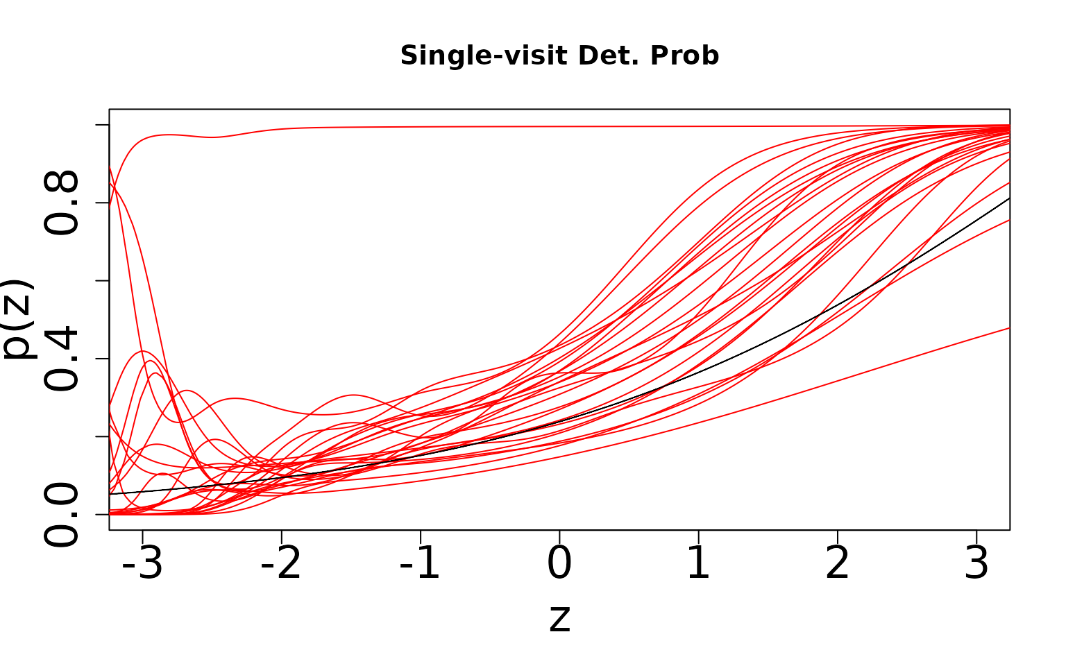
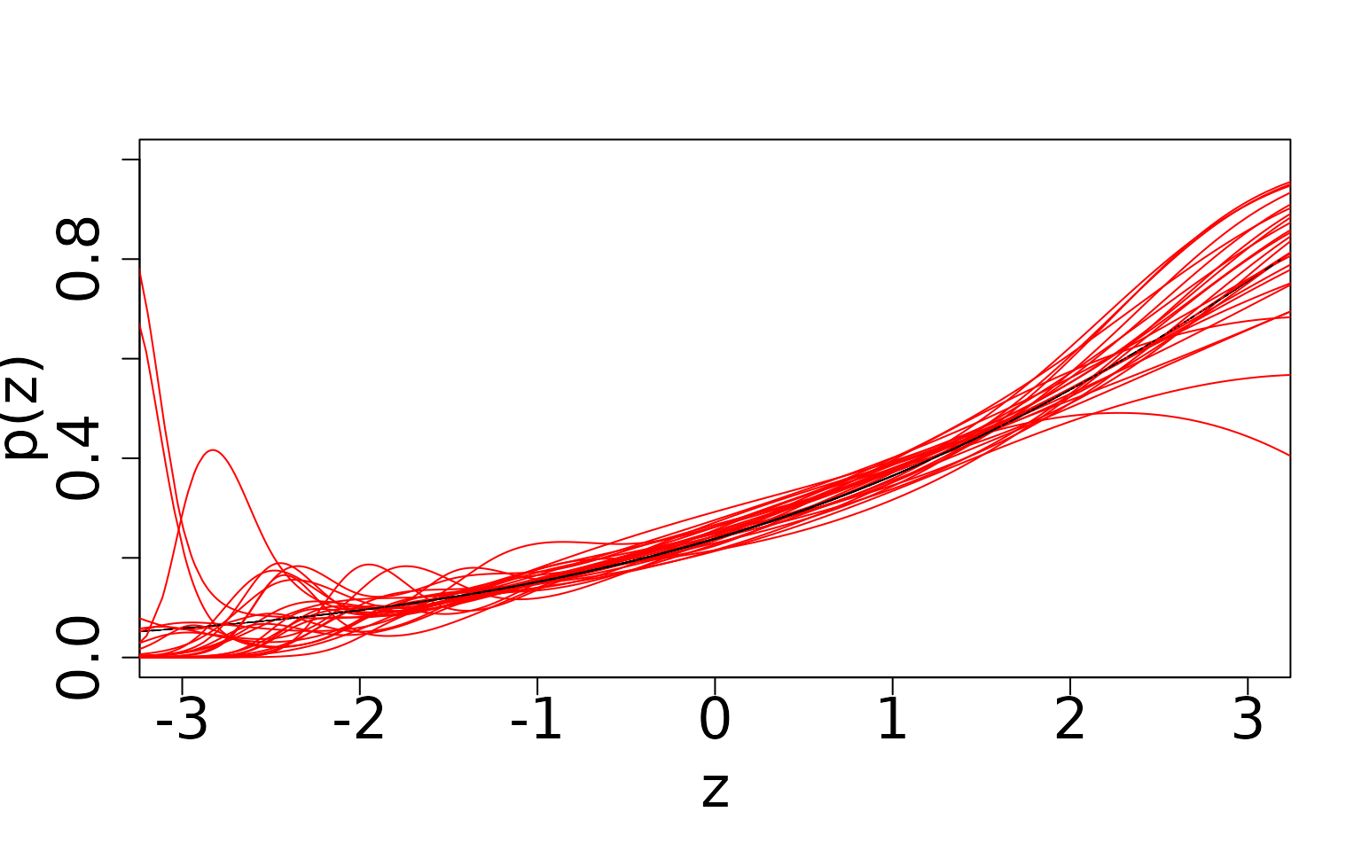
We can see that in the single visit case estimates of maximum occurrence and detection probabilities cover almost the whole range between 0 and 1. On average, occurrence probability is underestimated (i.e., majority of red lines fall below the black line), while detection probability is overestimated (i.e., majority of red lines fall above the black line).
Next we look at results from the double visit scenario.
occur_estDV <- detect_estDV <- X.sp <- X.p.sp <- vector("list", length(dv_dat_large))

for (i in 1:length(dv_dat_large)) {
  dat <- dv_dat_large[[i]]

  # Site x Replicate
  y <- dat$y[, , 1:2]
  # Occurrence Covariates
  X <- dat$X
  # Detection Covariates
  X.p <- dat$X.p

  # Create a spline basis for each covariate
  numKnots <- 7
  m <- 1:numKnots
  psiBound <- c(floor(min(X[, , 2])), ceiling(max(X[, , 2])))
  pBound <- c(floor(min(X.p[, , , 2])), ceiling(max(X.p[, , , 2])))

  X.sp[[i]] <- as.data.frame(bs(X[, , 2], knots = psiBound[1] + m * psiBound[2] / (numKnots + 1)))
  X.p.sp[[i]] <- bs(X.p[, , , 2], knots = pBound[1] + m * pBound[2] / (numKnots + 1))

  detectCovFormatted <- vector("list", numKnots + 3)
  for (j in 1:(numKnots + 3)) {
    detectCovFormatted[[j]] <- X.p.sp[[i]][, j]
  }

  names(X.sp[[i]]) <- paste("z", 1:(numKnots + 3), sep = "")
  names(detectCovFormatted) <- paste("p", 1:(numKnots + 3), sep = "")


  formattedData <- list(
    y = y, occ.covs = X.sp[[i]],
    det.covs = detectCovFormatted
  )


  occ.formula <- formula(paste("~", paste("z", 1:(numKnots + 3), sep = "", collapse = "+")))
  det.formula <- formula(paste("~", paste("p", 1:(numKnots + 3), sep = "", collapse = "+")))


  n.samples <- 5000
  n.burn <- 3000
  n.thin <- 2
  n.chains <- 3


  # Priors
  prior.list <- list(
    beta.normal = list(mean = 0, var = 100),
    alpha.normal = list(mean = 0, var = 100)
  )


  initsDV <- list(
    alpha = rep(0, length(formattedData$det.covs) + 1),
    beta = rep(0, ncol(formattedData$occ.covs) + 1), z = apply(formattedData$y, 1, max, na.rm = T)
  )

  out_dv <- PGOcc(
    occ.formula = occ.formula, det.formula = det.formula,
    data = formattedData,
    inits = initsDV, n.samples = n.samples, priors = prior.list,
    n.omp.threads = 1, verbose = F, n.report = 1000,
    n.burn = n.burn, n.thin = n.thin, n.chains = n.chains
  )

  occur_estDV[[i]] <- apply(out_dv$beta.samples, 2, mean) ## occurrence coeffs
  detect_estDV[[i]] <- apply(out_dv$alpha.samples, 2, mean) ## detection coeffs
}
dat <- dv_dat_large[[1]]
zData <- dat$X[, , 2]
psiData <- dat$psi[, 1]
idx <- order(zData)
thin <- 1:length(zData)
basisPsi <- X.sp[[1]]

plot((zData[idx])[thin], (psiData[idx])[thin], ylim = c(0, 1), type = "l", lwd = .5,
     xlim = c(-3, 3), xlab = "x", ylab = "", cex.axis = 2, cex.lab = 2,
     main = 'Double-visit Occ Prob')
for (i in 2:length(occur_estDV)) {
  dat <- dv_dat_large[[i]]
  zData <- dat$X[, , 2]
  psiData <- dat$psi[, 1]
  idx <- order(zData)
  thin <- 1:length(zData)
  basisPsi <- X.sp[[i]]
  lines((zData[idx])[thin], (psiData[idx])[thin], lwd = .5)
}

for (i in 1:length(dv_dat_large)) {
  dat <- dv_dat_large[[i]]
  zData <- dat$X[, , 2]
  psiData <- dat$psi[, 1]
  idx <- order(zData)
  thin <- 1:length(zData)
  basisPsi <- X.sp[[i]]
  fitted.val <- exp(occur_estDV[[i]][[1]] +
    occur_estDV[[i]][[2]] * basisPsi[, 1] +
    occur_estDV[[i]][[3]] * basisPsi[, 2] +
    occur_estDV[[i]][[4]] * basisPsi[, 3] +
    occur_estDV[[i]][[5]] * basisPsi[, 4] +
    occur_estDV[[i]][[6]] * basisPsi[, 5] +
    occur_estDV[[i]][[7]] * basisPsi[, 6]
    + occur_estDV[[i]][[8]] * basisPsi[, 7]
    + occur_estDV[[i]][[9]] * basisPsi[, 8]
    + occur_estDV[[i]][[10]] * basisPsi[, 9]
    + occur_estDV[[i]][[11]] * basisPsi[, 10]) / (1 + exp(occur_estDV[[i]][[1]] +
    occur_estDV[[i]][[2]] * basisPsi[, 1] +
    occur_estDV[[i]][[3]] * basisPsi[, 2] +
    occur_estDV[[i]][[4]] * basisPsi[, 3] +
    occur_estDV[[i]][[5]] * basisPsi[, 4] +
    occur_estDV[[i]][[6]] * basisPsi[, 5] +
    occur_estDV[[i]][[7]] * basisPsi[, 6]
    + occur_estDV[[i]][[8]] * basisPsi[, 7]
    + occur_estDV[[i]][[9]] * basisPsi[, 8]
    + occur_estDV[[i]][[10]] * basisPsi[, 9]
    + occur_estDV[[i]][[11]] * basisPsi[, 10]))

  lines((zData[idx]), (fitted.val[idx]), col = "red", cex = .5)
}


dat <- dv_dat_large[[1]]
zData <- dat$X[, , 2]
psiData <- dat$psi[, 1]
idx <- order(zData)
thin <- 1:length(zData)
basisPsi <- X.sp[[1]]
lines(sort(zData[thin]), sort(psiData[thin]))

mtext(
  text = expression(paste(psi, "(x)")),
  side = 2,
  line = 2.5, cex = 2
)
dat <- dv_dat_large[[1]]
mData <- dat$X.p[, , , 2]
pData <- dat$p[, , 1]
idx <- order(mData)
thin <- 1:length(mData)
basisP <- X.p.sp[[i]]

plot((mData[idx])[thin], (pData[idx])[thin], ylim = c(0, 1), type = "l",
     lwd = .5, xlim = c(-3, 3), xlab = "z", ylab = "",
     cex.axis = 2, cex.lab = 2, main = 'Double-visit Det. Prob')

for (i in 2:length(dv_dat_large)) {
  dat <- dv_dat_large[[i]]
  mData <- dat$X.p[, , , 2]
  pData <- dat$p[, , 1]
  idx <- order(mData)
  thin <- 1:length(mData)
  idx <- order(mData)
  lines((mData[idx])[thin], (pData[idx])[thin], lwd = .5)
}
for (i in 1:length(dv_dat_large)) {
  basisP <- X.p.sp[[i]]
  dat <- dv_dat_large[[i]]

  mData <- dat$X.p[, , , 2]
  pData <- dat$p[, , 1]


  fitted.val <- exp(detect_estDV[[i]][[1]] +
    detect_estDV[[i]][[2]] * basisP[, 1] +
    detect_estDV[[i]][[3]] * basisP[, 2] +
    detect_estDV[[i]][[4]] * basisP[, 3] +
    detect_estDV[[i]][[5]] * basisP[, 4] +
    detect_estDV[[i]][[6]] * basisP[, 5] +
    detect_estDV[[i]][[7]] * basisP[, 6]
    + detect_estDV[[i]][[8]] * basisP[, 7]
    + detect_estDV[[i]][[9]] * basisP[, 8]
    + detect_estDV[[i]][[10]] * basisP[, 9]
    + detect_estDV[[i]][[11]] * basisP[, 10]) / (1 + exp(detect_estDV[[i]][[1]] +
    detect_estDV[[i]][[2]] * basisP[, 1] +
    detect_estDV[[i]][[3]] * basisP[, 2] +
    detect_estDV[[i]][[4]] * basisP[, 3] +
    detect_estDV[[i]][[5]] * basisP[, 4] +
    detect_estDV[[i]][[6]] * basisP[, 5] +
    detect_estDV[[i]][[7]] * basisP[, 6]
    + detect_estDV[[i]][[8]] * basisP[, 7]
    + detect_estDV[[i]][[9]] * basisP[, 8]
    + detect_estDV[[i]][[10]] * basisP[, 9]
    + detect_estDV[[i]][[11]] * basisP[, 10]))


  idx <- order(mData)
  lines((mData[idx])[thin], (fitted.val[idx])[thin], col = "red", cex = .5)
}

dat <- dv_dat_large[[1]]
mData <- dat$X.p[, , , 2]
pData <- dat$p[, , 1]
idx <- order(mData)
thin <- 1:length(mData)
basisPSV <- X.p.sp[[i]]
lines((mData[idx])[thin], (pData[idx])[thin])


mtext(
  text = expression(paste(p, "(z)")),
  side = 2,
  line = 2.5, cex = 2
)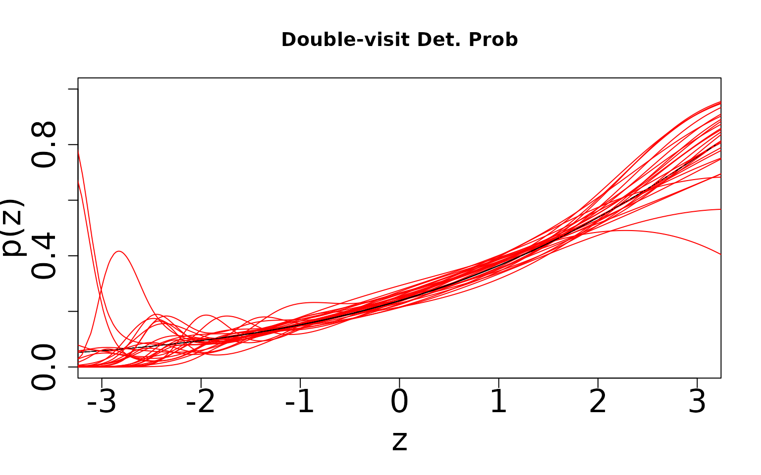
In contrast, with double visit data, there is a much narrower range, and the shape of the fit matches the truth much more clearly. As we mentioned in the single-visit case, we see “edge effects” as a result of simulating covariates with a standard normal distribution. We expect that as we increase the sample size further to an even more extreme scale, we would have enough instances of uncommon values of covariates at the tails to estimate this part of the curve more robustly.
Streamlining this workflow
This seems like a lot of pre-processing code. Is there an easier way
to investigate weak identifiability? Here are some helper functions for
pre-processing the data for input into a spOcc model
fitting procedure and for plotting the results. The plot functions can
be further adapted for different number of knots.
numKnots <- 7
dataToUse <- preprocess_data(sv_dat_large[[1]], numKnots)

occ.formula <- formula(paste("~", paste("z", 1:(numKnots + 3), sep = "", collapse = "+")))
det.formula <- formula(paste("~", paste("p", 1:(numKnots + 3), sep = "", collapse = "+")))


n.samples <- 5000
n.burn <- 3000
n.thin <- 2
n.chains <- 3


# Priors
prior.list <- list(
  beta.normal = list(mean = 0, var = 100),
  alpha.normal = list(mean = 0, var = 100)
)


initsSV <- list(
  alpha = rep(0, length(dataToUse$formattedData$det.covs) + 1),
  beta = rep(0, ncol(dataToUse$formattedData$occ.covs) + 1), z = as.vector(dataToUse$formattedData$y)
)

out_sv <- PGOcc(
  occ.formula = occ.formula, det.formula = det.formula,
  data = dataToUse$formattedData,
  inits = initsSV, n.samples = n.samples, priors = prior.list,
  n.omp.threads = 1, verbose = F, n.report = 1000,
  n.burn = n.burn, n.thin = n.thin, n.chains = n.chains
)

occur_est <- apply(out_sv$beta.samples, 2, mean) ## occurrence coeffs
detect_est <- apply(out_sv$alpha.samples, 2, mean) ## detection coeffs
Below we load in the results from the double visit simulations, which you can download yourself if you don’t want to run the full code (which can take a couple of hours). Note the single-visit results can also be downloaded by chaing the dv/DV to sv/SV in the file names below.
load(file = url("https://www.jeffdoser.com/files/misc/id-vignette/dv_dat_largeScaleEx.RData"))
load(file = url("https://www.jeffdoser.com/files/misc/id-vignette/occurDV_largeScaleEx.RData"))
load(file = url("https://www.jeffdoser.com/files/misc/id-vignette/basisPSiDV_largeScaleEx.RData"))

plot_occur(dv_dat_large, X.sp, occur_estDV)
load(file = url("https://www.jeffdoser.com/files/misc/id-vignette/detectDV_largeScaleEx.RData"))
load(file = url("https://www.jeffdoser.com/files/misc/id-vignette/basisPDV_largeScaleEx.RData"))

plot_detect(dv_dat_large, X.p.sp, detect_estDV)