Spatially varying coefficient models in spOccupancy
Jeffrey W. Doser
2022 (last update: July 25, 2023)
Source:vignettes/svcModels.Rmd
svcModels.RmdIntroduction
This vignette details spOccupancy functionality to fit
single-species and multi-species spatially varying coefficient (SVC)
models. Single-species models were introduced in v0.5.0 while
multi-species models were introduced in v0.7.0. When fitting models
across large spatial domains, it is increasingly likely that the effect
of spatial and/or temporal covariates on species occurrence varies
across space. Ignoring such spatial variability, or nonstationarity, can
result in reduced predictive performance and biased inference on the
effect of covariates at different spatial regions (Finley 2011; Rollinson et al. 2021). SVC
occupancy models are a flexible extension of spatial occupancy models
that allow for not only the intercept to vary across space, but also
allows the effects of the covariates themselves to vary spatially,
resulting in each spatial location having a unique effect of the
covariate (Pease, Pacifici, and Kays
2022). These models can generate key insights into how
environmental factors differentially influence species across its range,
how temporal trends vary across different parts of a species range, and
the relative importance of different covariate effects at different
parts of the species range.
Here we introduce six functions for fitting SVC models in
spOccupancy. The function svcPGOcc() fits a
single-season SVC occupancy model, and is an extension to the basic
spatial occupancy model fit by spPGOcc(). The function
svcTPGOcc() fits a multi-season SVC occupancy model, which
serves as an extension to the spatio-temporal occupancy model fit by
stPGOcc() where replicated detection-nondetection data are
collected over multiple primary time periods (i.e., breeding seasons,
years). Additionally, we include two functions for fitting SVC
generalized linear models (GLMs) where we ignore imperfect detection:
svcPGBinom() fits a single-season SVC GLM and
svcTPGBinom() fits a multi-species GLM. In these functions,
we also allow for modeling binomial data instead of the usual binary
detection-nondetection data, which may be applicable for certain species
or scenarios where imperfect detection may not be as large of an issue
(e.g., modeling tree species distributions using a nested plot/subplot
design). Lastly, we introduce two multi-species models,
svcMsPGOcc() and svcTMsPGOcc(), which fit
single-season and multi-season multi-species spatially varying
coefficient occupancy models, respectively.
As per usual, we use Pólya-Gamma data augmentation to yield a computationally efficient Gibbs sampler for GLM-type models with a logit link function (Polson, Scott, and Windle 2013), and use Nearest Neighbor Gaussian Processes (Datta et al. 2016) in all SVC models to greatly reduce the computational burden encountered when fitting models with spatial random effects formulated as a Gaussian process. The two multi-species models use a spatial factor modeling approach (Lopes and West 2004) to model the spatially varying effects for each species. This approach implicitly accounts for species correlations in both the residual spatial random effects and the effects of the spatially varying covariates themselves. See Doser, Finley, and Banerjee (2023) and Doser et al. (2024) for in depth statistical details on this approach.
In this vignette, we will walk through each of the four
single-species SVC models in spOccupancy, detailing how to
fit the models, do model comparison using the Widely Available
Information Criterion (WAIC) and/or k-fold cross-validation, as well as
make predictions across an area of interest to generate maps of the
spatially varying coefficients. We will work with simulated data sets
and will walk through how to simulate data sets using the
spOccupancy functions simOcc(),
simTOcc(), simBinom(),
simTBinom(), and simMsOcc(). We will not go
into explicit detail for some of the model-fitting function arguments
(e.g., priors, initial values) as the syntax is nearly identical to
other spOccupancy functions, so we encourage you to first
work through the spOccupancy
introductory vignette if you are not at least vaguely familiar with
spOccupancy syntax.
Below, we first load the spOccupancy package, as well as
the ggplot2 package to create some basic plots of our
results. We also set a seed so you can reproduce our results.
library(spOccupancy)
library(ggplot2)
set.seed(300)
Spatially varying coefficient occupancy model
Basic model description
Let \(\boldsymbol{s}_j\) denote the spatial coordinates of site \(j\), where \(j = 1, \dots, J\). We define \(z(\boldsymbol{s}_j)\) as the true presence (1) or absence (0) at site \(j\) with spatial coordinates \(\boldsymbol{s}_j\). We model \(z(\boldsymbol{s}_j)\) as
\[\begin{equation}\label{z} z(\boldsymbol{s}_j) \sim \text{Bernoulli}(\psi(\boldsymbol{s}_j)), \end{equation}\]
where \(\psi(\boldsymbol{s}_j)\) is the occurrence probability at site \(j\). We model \(\psi(\boldsymbol{s}_j)\) according to
\[\begin{equation}\label{psi} \text{logit}(\psi(\boldsymbol{s}_j)) = \textbf{x}(\boldsymbol{s}_j)\boldsymbol{\beta} + \tilde{\textbf{x}}(\boldsymbol{s}_j)\textbf{w}(\boldsymbol{s}_j), \end{equation}\]
where \(\boldsymbol{\beta}\) is a vector of \(H\) regression coefficients (including an intercept) that describe the non-spatial effects of covariates \(\textbf{x}(\boldsymbol{s}_j)\), and \(\textbf{w}(\boldsymbol{s}_j)\) is a vector of \(\tilde{H}\) spatially varying effects of covariates \(\tilde{\textbf{x}}(\boldsymbol{s}_j)\). Note that \(\tilde{\textbf{x}}(\boldsymbol{s}_j)\) may be identical to \(\textbf{x}(\boldsymbol{s}_j)\) if all covariates effects are assumed to vary spatially, or a subset of \(\textbf{x}(\boldsymbol{s}_j)\) if some effects are assumed to be constant across space. The model reduces to a traditional single-species occupancy model when all covariate effects are assumed constant across space and a spatial occupancy model (Johnson et al. 2013; Doser et al. 2022) when only the intercept is assumed to vary across space.
The spatially varying effects \(\textbf{w}(\boldsymbol{s}_j)\) serve as local adjustments of the covariate effects at site \(j\) from the overall non-spatial effects \(\boldsymbol{\beta}\), resulting in the covariate having a unique effect on species occurrence at each site \(j\). Following Gelfand et al. (2003), we model each \(h = 1, \dots, \tilde{H}\) spatially varying effect \(\text{w}_h(\boldsymbol{s}_j)\) using a zero-mean spatial Gaussian process. More specifically, we have
\[\begin{equation}\label{w} \text{$\text{w}_h(\boldsymbol{s})$} \sim N(\boldsymbol{0}, \boldsymbol{C}_h(\boldsymbol{s}, \boldsymbol{s}', \boldsymbol{\theta}_h)), \end{equation}\]
where \(\boldsymbol{C}_h(\boldsymbol{s}, \boldsymbol{s}', \boldsymbol{\theta}_h)\) is a \(J \times J\) covariance matrix that is a function of the distances between any pair of site coordinates \(\boldsymbol{s}\) and \(\boldsymbol{s}'\) and a set of parameters (\(\boldsymbol{\theta}_h\)) that govern the spatial process according to a spatial correlation function. Our associated software implementation supports four correlation functions: exponential, spherical, Gaussian, and Matern (Banerjee, Carlin, and Gelfand 2003). For the exponential, spherical, and Gaussian correlation functions, \(\boldsymbol{\theta}_h = \{\sigma^2_h, \phi_h\}\), where \(\sigma^2_h\) is a spatial variance parameter and \(\phi_h\) is a spatial decay parameter. Large values of \(\sigma^2_h\) indicate large variation in the magnitude of a covariate effect across space, while values of \(\sigma^2_h\) close to 0 suggests little spatial variability in the magnitude of the effect. \(\phi_h\) controls the range of the spatial dependence in the covariate effect and is inversely related to the spatial range, such that when \(\phi_h\) is small, the covariate effect has a larger range of spatial dependence and varies more smoothly across space compared to larger values of \(\phi_h\). The Matern correlation function has an additional smoothness parameter \(\nu_h\), which provides further flexibility in the smoothness and decay of the spatial process. To avoid the computational burden associated with fitting the full Gaussian process model, we use NNGPs as a computationally efficient and statistically robust alternative (Datta et al. 2016). See the supplemental material in the spOccupancy manuscript and Datta et al. (2016) for more details on NNGPs and their implementations in occupancy models.
To account for imperfect detection in an occupancy modeling framework (MacKenzie et al. 2002; Tyre et al. 2003), \(k = 1, \dots, K(\boldsymbol{s}_j)\) sampling replicates are obtained at each site \(j\). We model the observed detection (1) or nondetection (0) of a study species at site \(j\), denoted \(y_k(\boldsymbol{s}_j)\), conditional on the true latent occupancy process \(z(\boldsymbol{s}_j)\) following
\[\begin{equation}\label{yDet} y_{k}(\boldsymbol{s}_j) \mid z(\boldsymbol{s}_j) \sim \text{Bernoulli}(p_{k}(\boldsymbol{s}_j)z(\boldsymbol{s}_j)), \end{equation}\]
where \(p_k(\boldsymbol{s}_j)\) is the probability of detecting the species at site \(j\) during replicate \(k\) given the species is truly present at the site. We model detection probability as a function of site and/or observation-level covariates according to
\[\begin{equation}\label{pDet} \text{logit}(p_{k}(\boldsymbol{s}_j)) = \boldsymbol{v}_{k}(\boldsymbol{s}_j)\boldsymbol{\alpha}, \end{equation}\]
where \(\boldsymbol{\alpha}\) is a vector of regression coefficients (including an intercept) that describe the effect of site and/or observation covariates \(\boldsymbol{v}_{k}(\boldsymbol{s}_j)\) on detection.
To complete the Bayesian specification of the model, we assign Gaussian priors to the non-spatial occurrence and detection regression coefficients, an inverse-Gamma or uniform prior to the spatial variance parameters, and a uniform prior for the spatial decay (and smoothness if using a Matern correlation function) parameters.
Simulating data with simOcc()
The function simOcc() simulates single-species
detection-nondetection data. simOcc() has the following
arguments.
simOcc(J.x, J.y, n.rep, n.rep.max, beta, alpha, psi.RE = list(),
       p.RE = list(), sp = FALSE, svc.cols = 1, cov.model,
       sigma.sq, phi, nu, x.positive = FALSE, ...)
J.x and J.y indicate the number of spatial
locations to simulate data along a horizontal and vertical axis,
respectively, such that J.x * J.y is the total number of
sites (i.e., J). n.rep is a numeric vector of
length J that indicates the number of replicates at each of
the J sites (denoted as K in the previous model
description). n.rep.max is an optional value that can be
used to specify the maximum number of replicate surveys, which is useful
for emulating data from autonomous monitoring approaches (e.g., camera
traps) where sampling occurs over a set number of time periods (e.g.,
days), but any individual site was not sampled across all the time
periods. beta and alpha are numeric vectors
containing the intercept and any regression coefficient parameters for
the occurrence and detection portions of the occupancy model,
respectively. psi.RE and p.RE are lists that
are used to specify random intercepts on occurrence and detection,
respectively. These are only specified when we want to simulate data
with unstructured random intercepts. Each list should be comprised of
two tags: levels, a vector that specifies the number of
levels for each random effect included in the model, and
sigma.sq.psi or sigma.sq.p, which specify the
variances of the random effects for each random effect included in the
model. sp is a logical value indicating whether to simulate
data with at least one spatial Gaussian process for either the intercept
or some of the occupancy covariate effects. svc.cols is a
numeric vector indicating which of the covariates (including the
intercept) are generated with spatially varying effects. By default,
svc.cols = 1, which corresponds to a spatially varying
intercept when sp = TRUE (i.e., a spatial occupancy model).
cov.model specifies the covariance function used to model
the spatial dependence structure, with supported values of
exponential, matern, spherical,
and gaussian. Finally, sigma.sq is the spatial
variance parameter, phi is the spatial decay parameter, and
nu is the spatial smoothness parameter (only applicable
when cov.model = 'matern'). Note that
sigma.sq, phi, and nu should have
the same length as the number of spatially varying effects specified in
svc.cols. Lastly, the x.positive argument
indicates whether or not the occupancy covariates should be simulated to
be only positive from a Uniform(0, 1) distribution (TRUE)
or both positive and negative and simulated from a Normal(0, 1)
distribution (FALSE).
Below we simulate data across 1600 sites with anywhere between 1-4
replicates at a given site, a single covariate effect on occurrence, and
a single covariate effect on detection. We assume both the occupancy
intercept and the effect of the covariate vary across space, so we set
svc.cols = c(1, 2). We use a spherical correlation
function. We do not include any unstructured random effects on
occurrence or detection.
J.x <- 40
J.y <- 40
# Total number of sites
(J <- J.x * J.y)
[1] 1600
# Number of replicates at each site
n.rep <- sample(4:4, J, replace = TRUE)
# Intercept and covariate effect on occurrence
# Note these are the non-spatial effects.
beta <- c(-0.5, -0.2)
# Intercept and covariate effect on detection
alpha <- c(0.9, -0.3)
# No unstructured random intercept on occurrence
psi.RE <- list()
# No unstructured random intercept on detection
p.RE <- list()
# Spatial decay for intercept and covariate effect
phi <- c(3 / .8, 3 / .7)
# Spatial variance for intercept and covariate effect
sigma.sq <- c(1, 0.5)
# Simulate the occupancy covariate from a Normal(0, 1) distribution
x.positive <- FALSE
# Spatially varying coefficient columns
svc.cols <- c(1, 2)
# Simulate the data
dat <- simOcc(J.x = J.x, J.y = J.y, n.rep = n.rep, beta = beta,
              alpha = alpha, psi.RE = psi.RE, p.RE = p.RE,
              sp = TRUE, sigma.sq = sigma.sq, phi = phi,
              cov.model = 'spherical', svc.cols = svc.cols,
              x.positive = x.positive)
Next, let’s explore the simulated data a bit before we move on (plotting code adapted from Hooten and Hefley (2019)).
str(dat)List of 15
$ X : num [1:1600, 1:2] 1 1 1 1 1 1 1 1 1 1 ...
$ X.p : num [1:1600, 1:4, 1:2] 1 1 1 1 1 1 1 1 1 1 ...
$ coords : num [1:1600, 1:2] 0 0.0256 0.0513 0.0769 0.1026 ...
..- attr(*, "dimnames")=List of 2
.. ..$ : chr [1:1600] "1" "2" "3" "4" ...
.. ..$ : NULL
$ coords.full: num [1:1600, 1:2] 0 0.0256 0.0513 0.0769 0.1026 ...
..- attr(*, "dimnames")=List of 2
.. ..$ : NULL
.. ..$ : chr [1:2] "Var1" "Var2"
$ w : num [1:1600, 1:2] 0.266 0.658 -0.359 0.419 0.597 ...
$ w.grid : num [1:1600, 1:2] 0.266 0.658 -0.359 0.419 0.597 ...
$ psi : num [1:1600, 1] 0.423 0.819 0.318 0.448 0.442 ...
$ z : int [1:1600] 0 0 1 1 1 1 1 1 1 0 ...
$ p : num [1:1600, 1:4] NA NA NA NA 0.796 ...
$ y : int [1:1600, 1:4] NA NA NA NA 0 1 NA 0 1 0 ...
$ X.p.re : logi NA
$ X.re : logi NA
$ X.w : num [1:1600, 1:2] 1 1 1 1 1 1 1 1 1 1 ...
$ alpha.star : logi NA
$ beta.star : logi NAThe simulated data object consists of the following objects:
X (the occurrence design matrix), X.p (the
detection design matrix), coords (the spatial coordinates
of each site), w (the latent spatial process for any
covariates (and intercept) whose effects vary across space),
psi (occurrence probability), z (the latent
occupancy status), y (the detection-nondetection data),
X.w (the design matrix for the spatially varying
coefficients), X.p.re (the detection random effect levels
for each site), X.re (the occurrence random effect levels
for each site), alpha.star (the detection random effects
for each level of the random effect), beta.star (the
occurrence random effects for each level of the random effect). Note
because we did not include any unstructured effects on detection or
occurrence, the objects associated with the unstructured random effects
all have a value of NA.
# Detection-nondetection data
y <- dat$y
# Occurrence design matrix for fixed effects
X <- dat$X
# Detection design matrix for fixed effets
X.p <- dat$X.p
# Occurrence values
psi <- dat$psi
# Spatial coordinates
coords <- dat$coords
# Spatially varying intercept and covariate effects
w <- dat$w
# Simple plot of the occurrence probability across space.
# Dark points indicate high occurrence.
plot(coords, type = "n", xlab = "", ylab = "", asp = TRUE,
     main = "Simulated Occurrence", bty = 'n')
points(coords, pch=15, cex = 2.1, col = rgb(0,0,0,(psi-min(psi))/diff(range(psi))))
We see there is clear variation in occurrence probability across the simulated spatial region.
We can also visualize the spatially varying intercept and spatially
varying covariate effect. We do that by adding the spatial component of
the intercept and covariate effect (stored in the w matrix)
to the non-spatial components of the intercept and covariate effect
(stored in beta), and then visualizing using the same code
as before
# Intercept
int.effect <- beta[1] + w[, 1]
cov.effect <- beta[2] + w[, 2]
# Dark points indicate more positive effects, white points indicate more negative effects.
plot(coords, type = "n", xlab = "", ylab = "", asp = TRUE, main = "Intercept",
     bty = 'n')
points(coords, pch=15, cex = 2.1,
       col = rgb(0,0,0,(int.effect-min(int.effect))/diff(range(int.effect))))
plot(coords, type = "n", xlab = "", ylab = "", asp = TRUE, main = "Covariate Effect",
     bty = 'n')
points(coords, pch=15, cex = 2.1,
       col = rgb(0,0,0,(cov.effect-min(cov.effect))/diff(range(cov.effect))))
Note the spatial intercept corresponds fairly closely with the map of occurrence probability, which makes sense.
The final step before we can fit the model is to package up the data
in a list for use in spOccupancy model fitting functions.
This requires creating a list that consists of the
detection-nondetection data (y), occurrence covariates
(occ.covs), detection covariates (det.covs),
and coordinates (coords). See the introductory
vignette for more details. For our example here (and throughout the
vignette), we will fit the model to 75% of the data points (1200
locations) and subsequently predict at the remaining 400 values to show
the predictive ability of the model.
# Subset data for prediction.
# Split into fitting and prediction data set
pred.indx <- sample(1:J, round(J * .25), replace = FALSE)
y.fit <- y[-pred.indx, ]
y.pred <- y[pred.indx, ]
X.fit <- X[-pred.indx, ]
X.pred <- X[pred.indx, ]
X.p.fit <- X.p[-pred.indx, , ]
X.p.pred <- X.p[pred.indx, , ]
coords.fit <- coords[-pred.indx, ]
coords.pred <- coords[pred.indx, ]
psi.fit <- psi[-pred.indx]
psi.pred <- psi[pred.indx]
w.fit <- w[-pred.indx, ]
w.pred <- w[pred.indx, ]

# Package all data into a list
# Occurrence covariates
occ.covs <- X.fit[, 2, drop = FALSE]
colnames(occ.covs) <- c('occ.cov.1')
# Detection covariates
det.covs <- list(det.cov.1 = X.p.fit[, , 2])
# Package into a list for spOccupancy
data.list <- list(y = y.fit,
                  occ.covs = occ.covs,
                  det.covs = det.covs,
                  coords = coords.fit)
# Take a look at the data structure.
str(data.list)
List of 4
$ y : int [1:1200, 1:4] NA NA NA NA 0 1 NA 0 0 0 ...
$ occ.covs: num [1:1200, 1] 0.536 1.828 0.125 -0.254 -0.364 ...
..- attr(*, "dimnames")=List of 2
.. ..$ : NULL
.. ..$ : chr "occ.cov.1"
$ det.covs:List of 1
..$ det.cov.1: num [1:1200, 1:4] NA NA NA NA -1.53 ...
$ coords : num [1:1200, 1:2] 0 0.0256 0.0513 0.0769 0.1026 ...
..- attr(*, "dimnames")=List of 2
.. ..$ : chr [1:1200] "1" "2" "3" "4" ...
.. ..$ : NULLFitting spatially varying coefficient occupancy models with
svcPGOcc()
The function svcPGOcc() fits single-season SVC occupancy
models. svcPGOcc() has the following arguments:
svcPGOcc(occ.formula, det.formula, data, inits, priors,
         tuning, svc.cols = 1, cov.model = "exponential", NNGP = TRUE,
         n.neighbors = 15, search.type = "cb", n.batch,
         batch.length, accept.rate = 0.43,
         n.omp.threads = 1, verbose = TRUE, n.report = 100,
         n.burn = round(.10 * n.batch * batch.length),
         n.thin = 1, n.chains = 1, k.fold, k.fold.threads = 1,
         k.fold.seed = 100, k.fold.only = FALSE, ...)
The arguments to svcPGOcc() are identical as those for a
spatial occupancy model fit using spPGOcc(), with the
addition of the svc.cols argument to specify the SVCs in
the model. occ.formula and det.formula contain
the R model formulas for the occurrence and detection portions of the
occupancy model. Here we fit the model with a single covariate on both
occupancy and detection
occ.formula <- ~ occ.cov.1
det.formula <- ~ det.cov.1
The svc.cols argument is used to specify the covariates
whose effects are estimated as SVCs. svc.cols can either be
a numeric indexing vector with integer numbers corresponding to the
order in which you specified covariates in the occ.formula
argument, or can be a character vector with the names of the covariates
specified in occ.formula. Note that by default,
svc.cols = 1, which is equivalent to fitting a spatial
occupancy model with spPGOcc(). This clearly shows how SVC
occupancy models are a simple extension of a spatial occupancy model. A
spatial occupancy model is simply an SVC occupancy model where the only
spatially varying “covariate” is the intercept. If specifying
svc.cols as a character vector, use
'(Intercept)' to specify a spatially varying intercept.
Here we set svc.cols to include a spatially varying
intercept and spatially varying effect of the occurrence covariate. We
also specify the cov.model argument to indicate we will use
a spherical correlation function (note spOccupancy uses the
same correlation function for all SVCs). Usually, our default
correlation function is the exponential, which is what we use throughout
most of the other vignettes, but here we use a spherical correlation
function to show how spOccupancy can handle these other
functions.
svc.cols <- c(1, 2)
# OR
# svc.cols <- c('(Intercept)', 'occ.cov.1')
cov.model <- 'spherical'
We next specify the initial values, which are specified in a list
analogous to a spatial occupancy model using spPGOcc, with
the only difference being that if you supply initial values for the
spatial random effects w, these must be specified as a
two-dimensional matrix with rows corresponding to SVC and column
corresponding to site.
dist.data <- dist(data.list$coords)
inits.list <- list(alpha = 0, beta = 0, sigma.sq = 0.5,
                   phi = 3 / mean(dist.data),
                   z = apply(data.list$y, 1, max, na.rm = TRUE),
                   w = matrix(0, length(svc.cols), nrow(data.list$y)))
We next specify the priors to use for all parameters in the model
(alternatively, we could not specify priors and simply use
the default values svcPGOcc() provides). We will use the
default normal priors for the occurrence (beta) and
detection (alpha) regression coefficients. For the spatial
decay parameter (phi), we specify a uniform prior with
bounds based on the maximum and minimum inter-site distances. Our
default prior for phi is to set the lower bound to
3 / max and upper bound to 3 / min, where
max and min are the maximum and minimum
inter-site distances, respectively. This results in a prior that states
the effective spatial range is anywhere between the maximum distance
between sites and the smallest distance between sites. Lastly, we
specify an inverse-Gamma prior for sigma.sq. Following
Banerjee, Carlin, and Gelfand (2003), we
generally will set the scale parameter of the inverse-Gamma to 2 and the
shape parameter to our buest guess of the spatial variance. We could
also specify a uniform prior for the spatial variance parameter. For
binary data, very large values of sigma.sq can result in
undesirable and unrealistic values of the spatial random effects on the
logit scale, and so a uniform prior can be used to restrict
sigma.sq to some maximum value (e.g., 5) that is reasonable
on the logit scale (Wright et al.
2021).
priors.list <- list(alpha.normal = list(mean = 0, var = 2.72),
                    beta.normal = list(mean = 0, var = 2.72),
                    sigma.sq.ig = list(a = 2, b = 0.5),
                    phi.unif = list(a = 3 / max(dist.data),
                                    b = 3 / min(dist.data)))
The next three arguments (n.batch,
batch.length, and accept.rate) are all related
to the Adaptive MCMC sampler used when we fit the model. Updates for all
parameters with a uniform prior (in this case the spatial decay
parameter phi and the spatial variance parameter
sigma.sq) require the use of a Metropolis-Hastings
algorithm. We implement an adaptive Metropolis-Hastings algorithm as
discussed in Roberts and Rosenthal (2009).
This algorithm adjusts the tuning values for each parameter that
requires a Metropolis-Hastings update within the sampler itself. This
process results in a more efficient sampler than if we were to fix the
tuning parameters prior to fitting the model. The parameter
accept.rate is the target acceptance rate for each
parameter, and the algorithm will adjust the tuning parameters to hover
around this value. The default value is 0.43, which we suggest leaving
as is unless you have a good reason to change it. The tuning parameters
are updated after a single “batch”. We break up the total number of MCMC
samples into a set of “batches”, where each batch has a specific number
of samples. We must specify both the total number of batches
(n.batch) as well as the number of MCMC samples each batch
contains (batch.length). Thus, the total number of MCMC
samples is n.batch * batch.length. Typically, we set
batch.length = 25 and then play around with
n.batch until convergence is reached. Here we set
n.batch = 800 for a total of 20000 MCMC samples. We will
additionally specify a burn-in period of length 10000 and a thinning
rate of 10. We run the model for 3 chains, ultimately resulting in 3000
posterior samples. Importantly, we also need to specify an initial value
for the tuning parameters for the spatial decay parameter, spatial
variance parameter if using a uniform prior for sigma.sq,
and the smoothness parameter (if cov.model = 'matern').
These values are supplied as input in the form of a list with tags
phi, sigma.sq, and nu. The
initial tuning value can be any value greater than 0, but we recommend
starting the value out around 0.5. After some initial runs of the model,
if you notice the final acceptance rate of a parameter is much larger or
smaller than the target acceptance rate (accept.rate), you
can then change the initial tuning value to get closer to the target
rate. Here we set the initial tuning value for phi to 0.2
after some initial exploratory runs of the model.
batch.length <- 25
n.batch <- 800
n.burn <- 10000
n.thin <- 10
n.chains <- 1
tuning.list <- list(phi = 0.2)
We are now ready to run the model. We set the verbose
argument equal to TRUE and the n.report
argument to 100 to report progress on the MCMC chain after every 100th
batch. Additionally, we fit the model with an NNGP
(NNGP = TRUE) using 5 neighbors
(n.neighbors = 5). See the supplemental material in Doser et al. (2022) for more information on
choosing the number of neighbors in the NNGP approximation.
n.omp.threads <- 1
verbose <- TRUE
n.report <- 100 # Report progress at every 100th batch.
# Approx. run time: 2.4 min
out.svc <- svcPGOcc(occ.formula = occ.formula,
                    det.formula = det.formula,
                    data = data.list,
                    inits = inits.list,
                    n.batch = n.batch,
                    batch.length = batch.length,
                    priors = priors.list,
                    svc.cols = svc.cols,
                    cov.model = cov.model,
                    NNGP = TRUE,
                    n.neighbors = 5,
                    tuning = tuning.list,
                    n.report = n.report,
                    n.burn = n.burn,
                    n.thin = n.thin,
                    n.chains = n.chains)
----------------------------------------
Preparing to run the model
----------------------------------------
----------------------------------------
Building the neighbor list
----------------------------------------
----------------------------------------
Building the neighbors of neighbors list
----------------------------------------
----------------------------------------
Model description
----------------------------------------
NNGP Occupancy model with Polya-Gamma latent
variable fit with 1200 sites.
Samples per chain: 20000 (800 batches of length 25)
Burn-in: 10000
Thinning Rate: 10
Number of Chains: 1
Total Posterior Samples: 1000
Number of spatially-varying coefficients: 2
Using the spherical spatial correlation model.
Using 5 nearest neighbors.
Source compiled with OpenMP support and model fit using 1 thread(s).
Adaptive Metropolis with target acceptance rate: 43.0
----------------------------------------
Chain 1
----------------------------------------
Sampling ...
Batch: 100 of 800, 12.50%
Coefficient Parameter Acceptance Tuning
1 phi 40.0 0.21883
2 phi 60.0 0.26199
-------------------------------------------------
Batch: 200 of 800, 25.00%
Coefficient Parameter Acceptance Tuning
1 phi 48.0 0.22777
2 phi 24.0 0.18648
-------------------------------------------------
Batch: 300 of 800, 37.50%
Coefficient Parameter Acceptance Tuning
1 phi 48.0 0.19801
2 phi 44.0 0.17214
-------------------------------------------------
Batch: 400 of 800, 50.00%
Coefficient Parameter Acceptance Tuning
1 phi 20.0 0.16539
2 phi 64.0 0.21883
-------------------------------------------------
Batch: 500 of 800, 62.50%
Coefficient Parameter Acceptance Tuning
1 phi 48.0 0.20609
2 phi 44.0 0.22777
-------------------------------------------------
Batch: 600 of 800, 75.00%
Coefficient Parameter Acceptance Tuning
1 phi 48.0 0.19409
2 phi 32.0 0.17214
-------------------------------------------------
Batch: 700 of 800, 87.50%
Coefficient Parameter Acceptance Tuning
1 phi 20.0 0.18279
2 phi 48.0 0.24185
-------------------------------------------------
Batch: 800 of 800, 100.00%We can take a look at the model results using the
summary() function and compare them to the true values we
used to simulate the data.
summary(out.svc)
Call:
svcPGOcc(occ.formula = occ.formula, det.formula = det.formula,
    data = data.list, inits = inits.list, priors = priors.list,
    tuning = tuning.list, svc.cols = svc.cols, cov.model = cov.model,
    NNGP = TRUE, n.neighbors = 5, n.batch = n.batch, batch.length = batch.length,
    n.report = n.report, n.burn = n.burn, n.thin = n.thin, n.chains = n.chains)

Samples per Chain: 20000
Burn-in: 10000
Thinning Rate: 10
Number of Chains: 1
Total Posterior Samples: 1000
Run Time (min): 2.4247

Occurrence (logit scale):
               Mean     SD    2.5%     50%  97.5% Rhat ESS
(Intercept) -0.4588 0.2395 -0.8844 -0.4745 0.1194   NA  28
occ.cov.1   -0.1348 0.1711 -0.5139 -0.1249 0.2001   NA  38

Detection (logit scale):
               Mean     SD    2.5%     50%   97.5% Rhat  ESS
(Intercept)  0.8173 0.0756  0.6716  0.8169  0.9750   NA 1000
det.cov.1   -0.3330 0.0689 -0.4655 -0.3322 -0.2031   NA 1195

Spatial Covariance:
                       Mean     SD   2.5%    50%  97.5% Rhat ESS
sigma.sq-(Intercept) 1.1714 0.4789 0.4833 1.0988 2.2384   NA  35
sigma.sq-occ.cov.1   0.5152 0.2917 0.1688 0.4442 1.2236   NA  20
phi-(Intercept)      5.3224 1.5454 2.7013 5.2089 8.2520   NA  30
phi-occ.cov.1        5.0316 1.8285 2.3611 4.8531 9.1160   NA  13
# True values
beta
[1] -0.5 -0.2
alpha[1] 0.9 -0.3
sigma.sq[1] 1.0 0.5
phi[1] 3.750000 4.285714Because we only ran one chain of the model, we see the Rhat values are reported as NA. For a complete analysis, we would run the model for multiple chains, make sure the Rhat values are less than 1.1, and also ensure the effective sample sizes are adequately large. Here, the ESS values are somewhat low for the occurrence parameters and spatial covariance parameters, but we will continue interpreting the results for our exploratory purposes here. We see our model does a good job of recovering the true occurrence and detection regression coefficient values. The spatial variance parameters are also quite close to the estimated values. The spatial decay parameter value for the intercept is a bit larger than the simulated value. The spatial decay parameters are only weakly identifiable (i.e., there is very little information to estimate them), and thus estimating their true values can be a difficult task, in particular when fitting a model with multiple SVCs. Generally, we do not attempt to interpret the spatial decay parameters when fitting spatially-explicit occupancy models. Instead, we will often interpret the actual estimated spatial process values at each location, which are of particular interest in spatially varying coefficient models.
Next, let’s take a look at the resulting objects contained in the
out.svc list.
names(out.svc) [1] "rhat" "beta.samples" "alpha.samples" "theta.samples"
[5] "coords" "z.samples" "X" "X.re"
[9] "X.w" "w.samples" "psi.samples" "like.samples"
[13] "X.p" "X.p.re" "y" "ESS"
[17] "call" "n.samples" "n.neighbors" "cov.model.indx"
[21] "svc.cols" "type" "n.post" "n.thin"
[25] "n.burn" "n.chains" "pRE" "psiRE"
[29] "run.time" The resulting model object contains a variety of things, most of
which are just used in subsequent functions for posterior predictive
checks, prediction, and summarization. The objects that end in “samples”
are the posterior MCMC samples for the different objects. See
?svcPGOcc for more information.
To extract the estimates of the spatially varying coefficients at
each of the spatial locations in the data set used to fit the model, we
need to combine the non-spatial component of the coefficient (contained
in out.svc$beta.samples) and the spatial component of the
coefficient (contained in out.svc$w.samples). Recall that
in an SVC occupancy model, the total effect of a covariate at any given
location is the sum of the non-spatial effect and the adjustment of the
effect at that specific location. We provide the function
getSVCSamples() to extract the SVCs at each location.
svc.samples <- getSVCSamples(out.svc)
str(svc.samples)
List of 2
$ (Intercept): 'mcmc' num [1:1000, 1:1200] 0.721 -1.154 -0.956 -0.63 -0.453 ...
..- attr(*, "mcpar")= num [1:3] 1 1000 1
$ occ.cov.1 : 'mcmc' num [1:1000, 1:1200] -0.484 -0.759 -0.341 -0.805 -0.561 ...
..- attr(*, "mcpar")= num [1:3] 1 1000 1The resulting object, here called svc.samples, is a list
with each component corresponding to a matrix of the MCMC samples of
each spatially varying coefficient estimated in the model, with rows
corresponding to MCMC sample and column corresponding to site.
Below we plot the true SVCs for the covariate at the 1200 locations used for fitting the model compared to the mean estimates from our model.
# Get true covariate values at the locations used to fit the mdoel
cov.effect.fit <- beta[2] + w.fit[, 2]
# Get mean values of the SVC for the covariate
svc.cov.mean <- apply(svc.samples$occ.cov.1, 2, mean)
# Dark points indicate more positive effects, white points
# indicate more negative effects.
plot(coords.fit, type = "n", xlab = "", ylab = "", asp = TRUE,
     main = "True values", bty = 'n')
points(coords.fit, pch=15, cex = 2.1,
       col = rgb(0,0,0,(cov.effect.fit-min(cov.effect.fit))/diff(range(cov.effect.fit))))
plot(coords.fit, type = "n", xlab = "", ylab = "", asp = TRUE,
     main = "Estimated values", bty = 'n')
points(coords.fit, pch=15, cex = 2.1,
       col = rgb(0,0,0,(svc.cov.mean-min(svc.cov.mean))/diff(range(svc.cov.mean))))
Note that because we held out 400 random values across the study area, some of the white squares in the above image correspond to locations where we did not have any data (we will subsequently predict at these locations). We see our estimates align pretty closely with the true values used to simulate the data. Our mean estimates are smoother than the values used to generate the data. This is what we would expect, as the true values are a single instance of a simulated spatial process, whereas the mean values we have plotted average across individual instances to generate a more smoothed estimate. Overall, the model seems to accurately identify locations of low and high effects of the covariate.
Posterior Predictive Checks
The spOccupancy function ppcOcc() performs
a posterior predictive check for all spOccupancy model
objects as an assessment of Goodness of Fit (GoF). The key idea of GoF
testing is that a good model should generate data that closely align
with the observed data. If there are large differences in the observed
data from the model-generated data, our model is likely not very useful
(Hooten and Hobbs 2015). We can use the
ppcOcc() and summary() functions to generate a
Bayesian p-value as a quick assessment of model fit. A Bayesian p-value
that hovers around 0.5 indicates adequate model fit, while values less
than 0.1 or greater than 0.9 suggest our model does not fit the data
well. See the
introductory spOccupancy vignette and help page for
ppcOcc() for more details. Below we perform a posterior
predictive check with the Freeman-Tukey statistic, grouping the data by
individual sites.
Call:
ppcOcc(object = out.svc, fit.stat = "freeman-tukey", group = 1)

Samples per Chain: 20000
Burn-in: 10000
Thinning Rate: 10
Number of Chains: 1
Total Posterior Samples: 1000

Bayesian p-value:  0.503
Fit statistic:  freeman-tukey
We see our Bayesian p-value is very close to the optimal 0.5, suggesting adequate model fit (it would be a bit concerning if we didn’t see a good model fit here since we are using simulated data!).
Model Selection using WAIC
The spOccupancy function waicOcc()
calculates the Widely Applicable Information Criterion (WAIC) for all
spOccupancy fitted model objects. The WAIC is a fully
Bayesian information criterion that is adequate for comparing a set of
hierarchical models and selecting the best-performing model for final
analysis (see the
introductory spOccupancy vignette for more details).
Smaller values of WAIC indicate a better performing model. Below, we fit
a spatial occupancy model without the SVC of the covariate effect using
the spPGOcc() function (we could equivalently do this by
using svcPGOcc() and setting
svc.cols = 1).
# Using default priors and initial values.
# Approx. run time: 2.4 min
out.sp <- spPGOcc(occ.formula = occ.formula,
                  det.formula = det.formula,
                  data = data.list,
                  n.batch = n.batch,
                  batch.length = batch.length,
                  cov.model = cov.model,
                  NNGP = TRUE,
                  n.neighbors = 5,
                  tuning = tuning.list,
                  n.report = n.report,
                  n.burn = n.burn,
                  n.thin = n.thin,
                  n.chains = n.chains)
----------------------------------------
Preparing to run the model
----------------------------------------No prior specified for beta.normal.
Setting prior mean to 0 and prior variance to 2.72No prior specified for alpha.normal.
Setting prior mean to 0 and prior variance to 2.72No prior specified for phi.unif.
Setting uniform bounds based on the range of observed spatial coordinates.No prior specified for sigma.sq.
Using an inverse-Gamma prior with the shape parameter set to 2 and scale parameter to 1.z.inits is not specified in initial values.
Setting initial values based on observed databeta is not specified in initial values.
Setting initial values to random values from the prior distributionalpha is not specified in initial values.
Setting initial values to random values from the prior distributionphi is not specified in initial values.
Setting initial value to random value from the prior distributionsigma.sq is not specified in initial values.
Setting initial value to random value from the prior distributionw is not specified in initial values.
Setting initial value to 0----------------------------------------
Building the neighbor list
----------------------------------------
----------------------------------------
Building the neighbors of neighbors list
----------------------------------------
----------------------------------------
Model description
----------------------------------------
NNGP Occupancy model with Polya-Gamma latent
variable fit with 1200 sites.
Samples per chain: 20000 (800 batches of length 25)
Burn-in: 10000
Thinning Rate: 10
Number of Chains: 1
Total Posterior Samples: 1000
Using the spherical spatial correlation model.
Using 5 nearest neighbors.
Source compiled with OpenMP support and model fit using 1 thread(s).
Adaptive Metropolis with target acceptance rate: 43.0
----------------------------------------
Chain 1
----------------------------------------
Sampling ...
Batch: 100 of 800, 12.50%
Parameter Acceptance Tuning
phi 32.0 0.20201
-------------------------------------------------
Batch: 200 of 800, 25.00%
Parameter Acceptance Tuning
phi 40.0 0.23706
-------------------------------------------------
Batch: 300 of 800, 37.50%
Parameter Acceptance Tuning
phi 32.0 0.18279
-------------------------------------------------
Batch: 400 of 800, 50.00%
Parameter Acceptance Tuning
phi 68.0 0.27269
-------------------------------------------------
Batch: 500 of 800, 62.50%
Parameter Acceptance Tuning
phi 48.0 0.21025
-------------------------------------------------
Batch: 600 of 800, 75.00%
Parameter Acceptance Tuning
phi 44.0 0.18648
-------------------------------------------------
Batch: 700 of 800, 87.50%
Parameter Acceptance Tuning
phi 28.0 0.20201
-------------------------------------------------
Batch: 800 of 800, 100.00%
# WAIC for the SVC model
waicOcc(out.svc)
elpd pD WAIC
-1176.209 124.239 2600.896
# WAIC for the spatial occupancy model
waicOcc(out.sp)
elpd pD WAIC
-1220.89107 95.08627 2631.95468 We see the WAIC for the SVC occupancy model is lower than the WAIC for the spatial occupancy model, indicating the SVC model has improved model performance.
Prediction
Finally, we can use the predict() function with all
spOccupancy model-fitting functions to generate a series of
posterior predictive samples at new locations (as well as already
sampled locations), given a set of covariates and their spatial
locations. Note that we can predict both new occupancy values as well as
new detection values.
Below we predict occupancy probability at the 400 locations we held
out when fitting the model. The predict() function for
svcPGOcc() objects requires the model object, the design
matrix of covariates at the new locations (including the intercept if
specified in the model), and the spatial coordinates of the new
locations. Below we predict across the 400 “new” locations and plot them
in comparison to the true values we used to simulate the data.
# Take a look at X.pred, the design matrix for the prediction locations
head(X.pred)
[,1] [,2]
[1,] 1 0.2552401
[2,] 1 0.1139302
[3,] 1 1.4503029
[4,] 1 1.6331642
[5,] 1 0.2735918
[6,] 1 0.5891382
# Predict occupancy at the 400 new sites
out.pred <- predict(out.svc, X.pred, coords.pred)
----------------------------------------
Prediction description
----------------------------------------
NNGP Occupancy model with Polya-Gamma latent
variable fit with 1200 observations.
Number of covariates 2 (including intercept if specified).
Number of spatially-varying covariates 2 (including intercept if specified).
Using the spherical spatial correlation model.
Using 5 nearest neighbors.
Number of MCMC samples 1000.
Predicting at 400 non-sampled locations.
Source compiled with OpenMP support and model fit using 1 threads.
-------------------------------------------------
Predicting
-------------------------------------------------
Location: 100 of 400, 25.00%
Location: 200 of 400, 50.00%
Location: 300 of 400, 75.00%
Location: 400 of 400, 100.00%
Generating latent occupancy state
# Use the getSVCSamples() function to extract the SVC values
# at the prediction locations
svc.pred.samples <- getSVCSamples(out.svc, pred.object = out.pred)
# True covariate effect values at new locations
cov.effect.pred <- beta[2] + w.pred[, 2]
# Get mean values of the SVC for the covariate
svc.cov.pred.mean <- apply(svc.pred.samples$occ.cov.1, 2, mean)
# Dark points indicate more positive effects, white points indicate more
# negative effects.
plot(coords.pred, type = "n", xlab = "", ylab = "", asp = TRUE,
     main = "True values", bty = 'n')
points(coords.pred, pch=15, cex = 2.1,
       col = rgb(0,0,0,(cov.effect.pred-min(cov.effect.pred))/
                        diff(range(cov.effect.pred))))
plot(coords.pred, type = "n", xlab = "", ylab = "", asp = TRUE,
     main = "Estimated values", bty = 'n')
points(coords.pred, pch=15, cex = 2.1,
       col = rgb(0,0,0,(svc.cov.pred.mean-min(svc.cov.pred.mean))/
                        diff(range(svc.cov.pred.mean))))
           used  (Mb) gc trigger  (Mb) max used  (Mb)
Ncells  2466690 131.8    4585492 244.9  4585492 244.9
Vcells 13073124  99.8   40566458 309.5 50621557 386.3
We see a pretty close correspondence between the true values and the predicted values.
Spatially varying coefficient generalized linear model
Accounting for imperfect detection explicitly in an occupancy modeling framework may not be feasible given the data. In particular, single-visit (or nonreplicated) detection-nondetection data are a very common data source due to the extra expenses of doing multiple surveys at a given location. In this case, we cannot separately estimate imperfect detection from occupancy probability in an occupancy modeling framework without making strict assumptions (Lele, Moreno, and Bayne 2012), and so instead we might fit a more standard generalized linear model (GLM).
Additionally, occupancy models are much less frequently used for modeling plant species distributions than animal distributions. While imperfect detection is still prevalent in plant distribution studies (Chen et al. 2013), we may wish to model plant distribution data using a standard generalized linear modeling framework, in particular if we do not have replicate surveys available in our data set. If our inference focuses solely on the effects of covariates on where a species occurs and not the overall estimates of “occupancy probability”, this may be a feasible approach. However, all inferences made from such models that ignore imperfect detection should carefully consider how detection probability may vary across space and/or time, and what consequences this has on the interpretation of the results. For example, if a spatially varying covariate influences both the probability a species occurs at a location and the probability the species is detected, one would interpret the effect of the covariate as the effect on the confounded process of detection/occupancy probability.
Basic model description
As before, let \(y_k(\boldsymbol{s}_j)\) be the detection (1) or non-detection (0) of our species of interest at site \(j\) with spatial coordinates \(\boldsymbol{s}_j\). When not explicitly accounting for imperfect detection in an occupancy model, we will model the detection-nondetection data directly in a SVC GLM framework. Specifically, we have
\[\begin{equation}\label{yNoDet} y^*(\boldsymbol{s}_j) \sim \text{Binomial}(K(\boldsymbol{s}_j), \psi(\boldsymbol{s}_j)), \end{equation}\]
where \(y^*(\boldsymbol{s}_j) = \sum_{k = 1}^{K(\boldsymbol{s}_j)}y_{k}(\boldsymbol{s}_j)\), \(K(\boldsymbol{s}_j)\) is the number of replicate surveys at site \(j\), and \(\boldsymbol{\psi}(\boldsymbol{s}_j)\) is the occurrence probability at site \(j\). When only one replicate survey is available at each site, the Binomial likelihood in the previous equation reduces to a Bernoulli likelihood. We model \(\psi(\boldsymbol{s}_j)\) as before. Note that we can incorporate spatially varying covariates in the model of \(\psi(\boldsymbol{s}_j)\) that may influence detection probability of the species, but our estimates of \(\psi(\boldsymbol{s}_j)\) are still interpreted as relative occurrence probabilities.
Simulating data with simBinom()
The function simBinom() simulates single-species
detection-nondetection data for which detection is assumed perfect.
simBinom() has the following arguments, which are very
similar to those we saw previously with simOcc().
simBinom(J.x, J.y, weights, beta, psi.RE = list(),
         sp = FALSE, svc.cols = 1, cov.model, sigma.sq, phi, nu,
         x.positive = FALSE, ...)
J.x and J.y indicate the number of spatial
locations to simulate data along a horizontal and vertical axis,
respectively, such that J.x * J.y is the total number of
sites (i.e., J). weights is a numeric vector
of length J that indicates the number of Bernoulli trials
(replicates) at each of the J sites (denoted as K in the
previous model description). beta is a numeric vector
containing the intercept and any regression coefficient parameters for
the model, respectively. psi.RE is a list that is used to
specify unstructured random intercepts, respectively. These are only
specified when we want to simulate data with random intercepts. All
other arguments are the same as those we saw simOcc().
We simulate data across 1600 sites where we assume there is only a
single replicate survey at a given site and a single covariate effect on
relative occurrence. We assume both the intercept and the effect of the
covariate vary across space, so we set svc.cols = c(1, 2).
We use an exponential correlation function. We do not include any
unstructured random effects on occurrence or detection.
# Set seed again to get the same data set
set.seed(488)
J.x <- 40
J.y <- 40
# Total number of sites
(J <- J.x * J.y)
[1] 1600
# Number of replicates at each site
weights <- rep(1, J)
# Intercept and covariate effect
# Note these are the non-spatial effects.
beta <- c(-0.5, -0.2)
# No unstructured random intercepts
psi.RE <- list()
# Spatial decay for intercept and covariate effect
phi <- c(3 / .8, 3 / .7)
# Spatial variance for intercept and covariate effect
sigma.sq <- c(1, 0.5)
# Simulate the covariate from a Normal(0, 1) distribution
x.positive <- FALSE
# Spatially varying coefficient columns
svc.cols <- c(1, 2)
# Simulate the data
dat <- simBinom(J.x = J.x, J.y = J.y, weights = weights, beta = beta,
                psi.RE = psi.RE, sp = TRUE, sigma.sq = sigma.sq, phi = phi,
                cov.model = 'exponential', svc.cols = svc.cols,
                x.positive = x.positive)
Next, let’s explore the simulated data a bit before we move on (plotting code adapted from Hooten and Hefley (2019)).
str(dat)List of 8
$ X : num [1:1600, 1:2] 1 1 1 1 1 1 1 1 1 1 ...
$ coords : num [1:1600, 1:2] 0 0.0256 0.0513 0.0769 0.1026 ...
..- attr(*, "dimnames")=List of 2
.. ..$ : NULL
.. ..$ : chr [1:2] "Var1" "Var2"
$ w : num [1:1600, 1:2] 0.61481 0.00417 -0.26095 -0.54444 -0.9741 ...
$ psi : num [1:1600, 1] 0.539 0.362 0.402 0.338 0.329 ...
$ y : int [1:1600] 0 1 0 1 0 0 0 0 1 0 ...
$ X.re : logi NA
$ X.w : num [1:1600, 1:2] 1 1 1 1 1 1 1 1 1 1 ...
$ beta.star: logi NAThe simulated data object consists of the following objects:
X (the design matrix), coords (the spatial
coordinates of each site), w (the latent spatial process
for any covariates (and intercept) whose effects vary across space),
psi (relative occurrence probability), y (the
detection-nondetection data), X.w (the design matrix for
the spatially varying coefficients), X.re (the occurrence
random effect levels for each site), beta.star (the random
effects for each level of the unstructured random effect). Note because
we did not include any unstructured effects, the objects associated with
the unstructured random effects all have a value of NA.
# Detection-nondetection data
y <- dat$y
# Design matrix
X <- dat$X
# Occurrence values
psi <- dat$psi
# Spatial coordinates
coords <- dat$coords
# Spatially varying intercept and covariate effects
w <- dat$w
# Simple plot of the relative occurrence probability across space.
# Dark points indicate high occurrence.
plot(coords, type = "n", xlab = "", ylab = "", asp = TRUE,
     main = "Simulated Occurrence", bty = 'n')
points(coords, pch=15, cex = 2.1, col = rgb(0,0,0,(psi-min(psi))/diff(range(psi))))
Lastly, we package the data up in a list for use in
spOccupancy model fitting functions. For SVC GLMs, this
requires creating a list that consists of the detection-nondetection
data (y), covariates (covs), the binomial
weights aka the number of replicates (weights), and
coordinates (coords). Note that the covariates here are
stored in a single matrix object covs rather than split
apart into the occurrence (occ.covs) and detection
(det.covs) covariates as we do for occupancy models. As we
did for the SVC occupancy model, we will fit the model to 75% of the
data points (1200 locations) and subsequently predict at the remaining
400 values to show the predictive ability of the model.
# Subset data for prediction.
# Split into fitting and prediction data set
pred.indx <- sample(1:J, round(J * .25), replace = FALSE)
y.fit <- y[-pred.indx]
y.pred <- y[pred.indx]
X.fit <- X[-pred.indx, ]
X.pred <- X[pred.indx, ]
coords.fit <- coords[-pred.indx, ]
coords.pred <- coords[pred.indx, ]
psi.fit <- psi[-pred.indx]
psi.pred <- psi[pred.indx]
w.fit <- w[-pred.indx, ]
w.pred <- w[pred.indx, ]
weights.fit <- weights[-pred.indx]
weights.pred <- weights[pred.indx]

# Package all data into a list
# Covariates
covs <- X.fit[, 2, drop = FALSE]
colnames(covs) <- c('cov.1')
# Package into a list for spOccupancy
data.list <- list(y = y.fit,
                  covs = covs,
                  coords = coords.fit,
                  weights = weights.fit)
# Take a look at the data structure.
str(data.list)
List of 4
$ y : int [1:1200] 0 1 0 0 0 0 1 1 0 1 ...
$ covs : num [1:1200, 1] -0.178 0.791 0.733 -1.758 1.847 ...
..- attr(*, "dimnames")=List of 2
.. ..$ : NULL
.. ..$ : chr "cov.1"
$ coords : num [1:1200, 1:2] 0 0.0256 0.0513 0.1026 0.1282 ...
..- attr(*, "dimnames")=List of 2
.. ..$ : NULL
.. ..$ : chr [1:2] "Var1" "Var2"
$ weights: num [1:1200] 1 1 1 1 1 1 1 1 1 1 ...Fitting spatially varying coefficient generalized linear models with
svcPGBinom()
The function svcPGBinom() fits single-season SVC GLMs.
svcPGBinom() has the following arguments, which are nearly
identical to those we saw with svcPGOcc():
svcPGBinom(formula, data, inits, priors, tuning, svc.cols = 1,
           cov.model = "exponential", NNGP = TRUE,
           n.neighbors = 15, search.type = "cb", n.batch,
           batch.length, accept.rate = 0.43,
           n.omp.threads = 1, verbose = TRUE, n.report = 100,
           n.burn = round(.10 * n.batch * batch.length),
           n.thin = 1, n.chains = 1, k.fold, k.fold.threads = 1,
           k.fold.seed = 100, k.fold.only = FALSE, ...)
The only difference between the arguments of
svcPGBinom() and svcPGOcc() is that now we
only specify a single formula, formula, since we do not
separately model detection probability from occurrence probability.
Below we specify the formula, including the single covariate we
simulated the data with.
formula <- ~ cov.1As before, the svc.cols argument specifies the
covariates whose effects are estimated as SVCs. Here we set
svc.cols to include a spatially varying intercept and
spatially varying effect of the covariate. We also specify the
cov.model argument to indicate we will use an exponential
correlation function.
svc.cols <- c(1, 2)
cov.model <- 'exponential'
We next specify the initial values, which is exactly analogous to
svcPGOcc(), but we don’t have any initial values for the
detection parameters or the latent occupancy values, since we don’t
estimate those in an SVC GLM.
dist.data <- dist(data.list$coords)
inits.list <- list(beta = 0, sigma.sq = 0.5,
                   phi = 3 / mean(dist.data),
                   w = matrix(0, length(svc.cols), length(data.list$y)))
We next specify the priors to use for all parameters in the model,
which we set to be the same as those we used for
svcPGOcc().
priors.list <- list(beta.normal = list(mean = 0, var = 2.72),
                    sigma.sq.ig = list(a = 2, b = 0.5),
                    phi.unif = list(a = 3 / max(dist.data),
                                    b = 3 / min(dist.data)))
Finally, we specify the MCMC criteria exactly as we saw previously and then we are all set to run the model.
batch.length <- 25
n.batch <- 800
n.burn <- 10000
n.thin <- 10
n.chains <- 1
tuning.list <- list(phi = 0.2, sigma.sq = 0.2)
n.omp.threads <- 1
verbose <- TRUE
n.report <- 100 # Report progress at every 100th batch.
# Approx. run time: 1.8 min
out.svc <- svcPGBinom(formula = formula,
                      data = data.list,
                      inits = inits.list,
                      n.batch = n.batch,
                      batch.length = batch.length,
                      priors = priors.list,
                      svc.cols = svc.cols,
                      cov.model = cov.model,
                      NNGP = TRUE,
                      n.neighbors = 5,
                      tuning = tuning.list,
                      n.report = n.report,
                      n.burn = n.burn,
                      n.thin = n.thin,
                      n.chains = n.chains)
----------------------------------------
Preparing to run the model
----------------------------------------
----------------------------------------
Building the neighbor list
----------------------------------------
----------------------------------------
Building the neighbors of neighbors list
----------------------------------------
----------------------------------------
Model description
----------------------------------------
Spatial NNGP Binomial model with Polya-Gamma latent
variable fit with 1200 sites.
Samples per chain: 20000 (800 batches of length 25)
Burn-in: 10000
Thinning Rate: 10
Number of Chains: 1
Total Posterior Samples: 1000
Number of spatially-varying coefficients: 2
Using the exponential spatial correlation model.
Using 5 nearest neighbors.
Source compiled with OpenMP support and model fit using 1 thread(s).
Adaptive Metropolis with target acceptance rate: 43.0
----------------------------------------
Chain 1
----------------------------------------
Sampling ...
Batch: 100 of 800, 12.50%
Coefficient Parameter Acceptance Tuning
1 phi 36.0 0.18648
2 phi 24.0 0.22326
-------------------------------------------------
Batch: 200 of 800, 25.00%
Coefficient Parameter Acceptance Tuning
1 phi 40.0 0.16539
2 phi 44.0 0.16873
-------------------------------------------------
Batch: 300 of 800, 37.50%
Coefficient Parameter Acceptance Tuning
1 phi 52.0 0.17562
2 phi 44.0 0.17917
-------------------------------------------------
Batch: 400 of 800, 50.00%
Coefficient Parameter Acceptance Tuning
1 phi 24.0 0.22777
2 phi 28.0 0.17214
-------------------------------------------------
Batch: 500 of 800, 62.50%
Coefficient Parameter Acceptance Tuning
1 phi 76.0 0.20201
2 phi 32.0 0.17214
-------------------------------------------------
Batch: 600 of 800, 75.00%
Coefficient Parameter Acceptance Tuning
1 phi 44.0 0.15891
2 phi 68.0 0.20609
-------------------------------------------------
Batch: 700 of 800, 87.50%
Coefficient Parameter Acceptance Tuning
1 phi 48.0 0.19025
2 phi 36.0 0.19409
-------------------------------------------------
Batch: 800 of 800, 100.00%
# Compare to values used to generate the data
summary(out.svc)
Call:
svcPGBinom(formula = formula, data = data.list, inits = inits.list,
    priors = priors.list, tuning = tuning.list, svc.cols = svc.cols,
    cov.model = cov.model, NNGP = TRUE, n.neighbors = 5, n.batch = n.batch,
    batch.length = batch.length, n.report = n.report, n.burn = n.burn,
    n.thin = n.thin, n.chains = n.chains)

Samples per Chain: 20000
Burn-in: 10000
Thinning Rate: 10
Number of Chains: 1
Total Posterior Samples: 1000
Run Time (min): 1.891

Occurrence (logit scale):
               Mean     SD    2.5%     50%  97.5% Rhat ESS
(Intercept) -0.2728 0.1473 -0.5770 -0.2596 0.0057   NA  34
cov.1        0.0831 0.1470 -0.2261  0.0913 0.3611   NA  22

Spatial Covariance:
                        Mean      SD   2.5%    50%   97.5% Rhat ESS
sigma.sq-(Intercept)  0.3826  0.1631 0.1793 0.3473  0.8226   NA  31
sigma.sq-cov.1        0.2842  0.1788 0.0846 0.2438  0.8155   NA  14
phi-(Intercept)       6.8393  2.6174 2.8451 6.4441 13.8589   NA  27
phi-cov.1            14.9416 15.3815 2.7489 9.4919 66.0294   NA  10
# True values
beta
[1] -0.5 -0.2
sigma.sq[1] 1.0 0.5
phi[1] 3.750000 4.285714Let’s next extract the full SVC values using the
getSVCSamples() function and then compare the estimated
values to those used to generate the model. This time, we won’t make a
map of the predicted values, but rather will just look at a scatter plot
of fitted values vs. true values.
# Intercept ---------------------------------------------------------------
svc.samples <- getSVCSamples(out.svc)
int.quants <- apply(svc.samples[["(Intercept)"]], 2,
                    quantile, probs = c(0.025, 0.5, 0.975))
svc.true.fit <- beta + w.fit
plot(svc.true.fit[, 1], int.quants[2, ], pch = 19,
     ylim = c(min(int.quants[1, ]), max(int.quants[3, ])),
     xlab = "True", ylab = "Fit", main = 'Intercept')
abline(0, 1)
arrows(svc.true.fit[, 1], int.quants[2, ], svc.true.fit[, 1],
       col = 'gray', int.quants[1, ], length = 0.02, angle = 90)
arrows(svc.true.fit[, 1], int.quants[1, ], svc.true.fit[, 1],
       col = 'gray', int.quants[3, ], length = 0.02, angle = 90)
points(svc.true.fit[, 1], int.quants[2, ], pch = 19)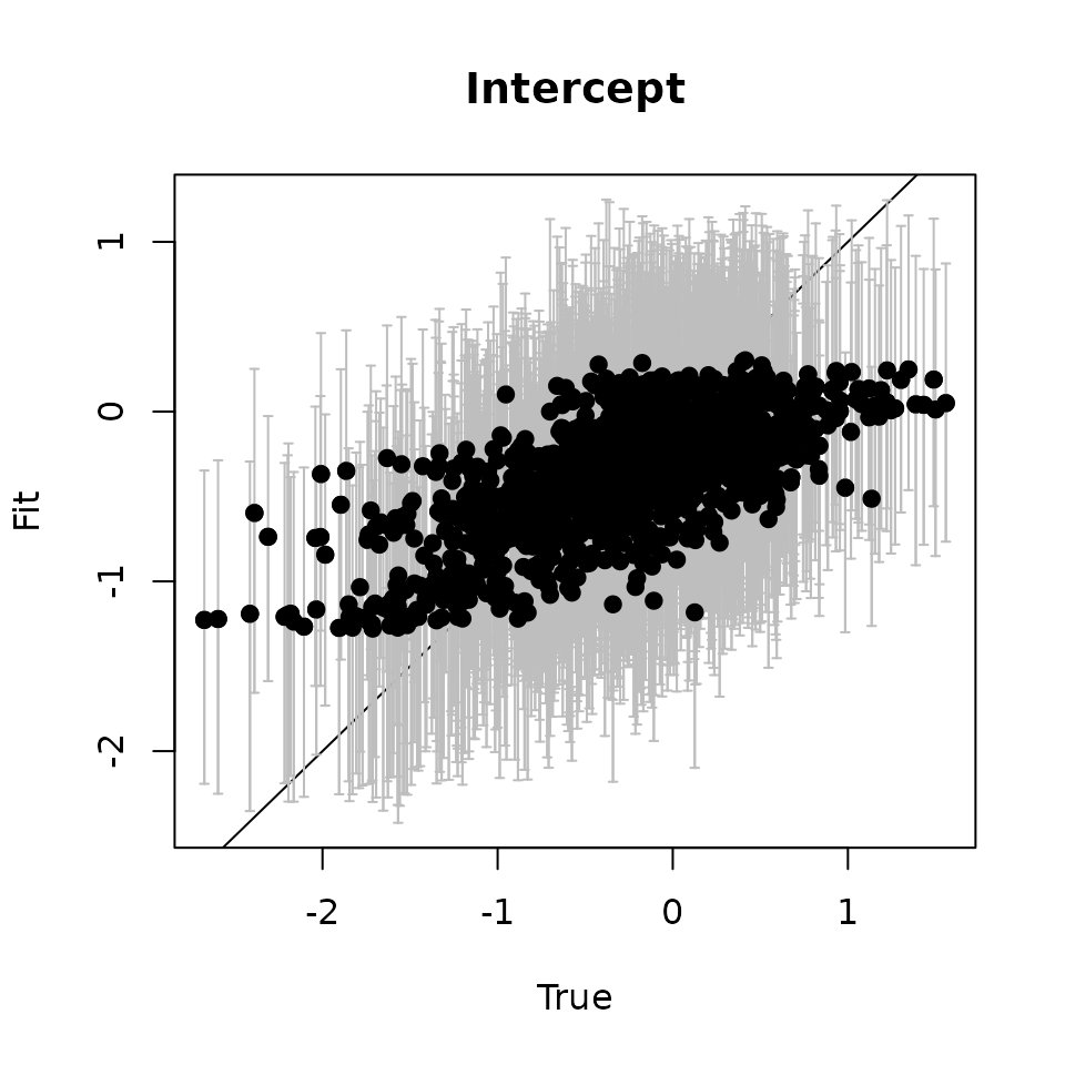
# Covariate ---------------------------
cov.quants <- apply(svc.samples[["cov.1"]], 2, quantile,
                    probs = c(0.025, 0.5, 0.975))
svc.true.fit <- beta + w.fit
plot(svc.true.fit[, 2], cov.quants[2, ], pch = 19,
     ylim = c(min(cov.quants[1, ]), max(cov.quants[3, ])),
     xlab = "True", ylab = "Fit", main = 'Covariate')
abline(0, 1)
arrows(svc.true.fit[, 2], cov.quants[2, ], svc.true.fit[, 2],
       col = 'gray', cov.quants[1, ], length = 0.02, angle = 90)
arrows(svc.true.fit[, 2], cov.quants[1, ], svc.true.fit[, 2],
       col = 'gray', cov.quants[3, ], length = 0.02, angle = 90)
points(svc.true.fit[, 2], cov.quants[2, ], pch = 19)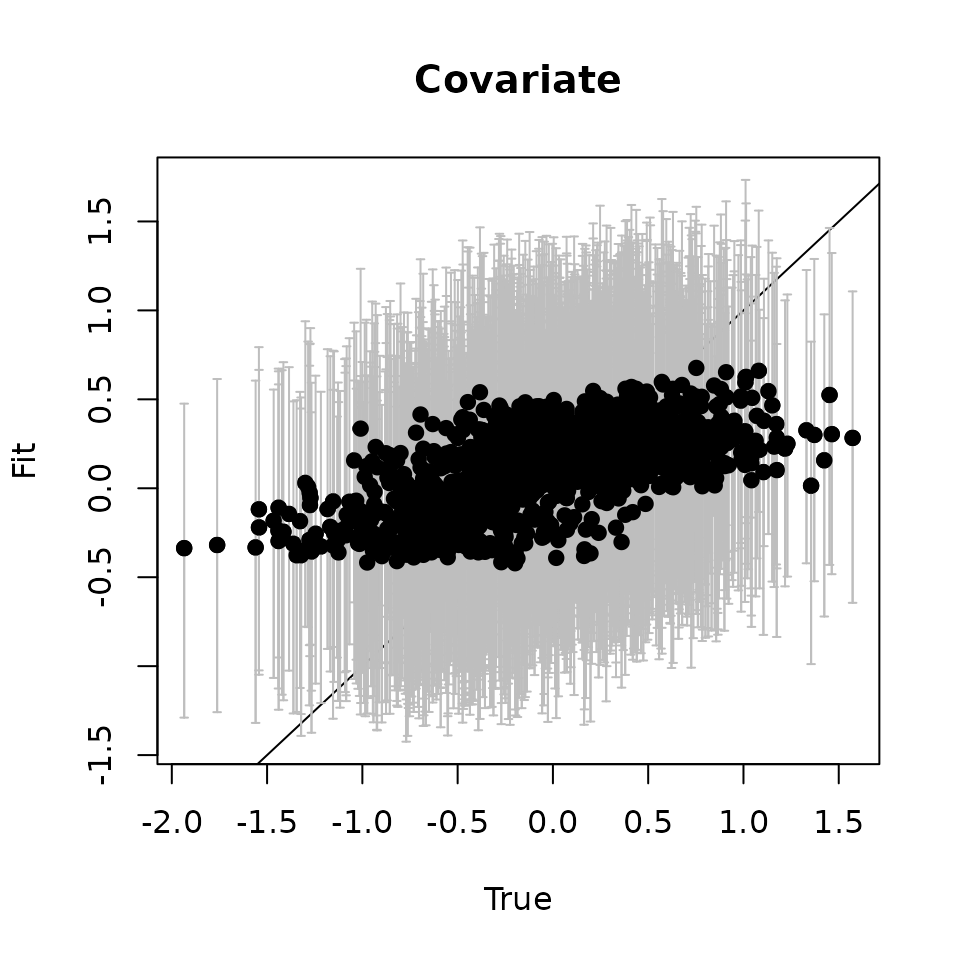
Here we see our estimated values capture the patterns in the simulated values. Notice that the estimated values do not fall exactly on the one to one line, and rather the estimated values are all seemingly closer to zero than the true values, in particular for the sites that have a large magnitude of the effect. This is a common phenomenon in spatial models that use binary data in a GLM framework as a result of the lack of information in binary data as well as the link function (e.g., logit) that transforms binary data to the real scale. Generally, as the number of spatial locations increase and the spatial range increases (i.e., the spatial decay parameter \(\phi\) gets smaller), we will tend to see the values be more closely approximated by the model. Regardless, we generally see good coverage of the 95% credible intervals for the true values (ideally we want 95% of the gray lines to overlap the black one to one line), and the estimated means capture the pattern in the effects across space.
Model selection using WAIC
We can do model selection using WAIC as we saw with
svcPGOcc(). Below we fit a spatial GLM that assumes the
covariate effect is stationary across the study area. We then compare
the two models with WAIC.
out.glm <- svcPGBinom(formula = formula,
                      data = data.list,
                      n.batch = n.batch,
                      batch.length = batch.length,
                      svc.cols = 1,
                      cov.model = cov.model,
                      NNGP = TRUE,
                      n.neighbors = 5,
                      tuning = tuning.list,
                      n.report = n.report,
                      n.burn = n.burn,
                      n.thin = n.thin,
                      n.chains = n.chains)
----------------------------------------
Preparing to run the model
----------------------------------------No prior specified for beta.normal.
Setting prior mean to 0 and prior variance to 2.72No prior specified for phi.unif.
Setting uniform bounds based on the range of observed spatial coordinates.No prior specified for sigma.sq.
Using an inverse-Gamma prior with the shape parameter set to 2 and scale parameter to 1.beta is not specified in initial values.
Setting initial values to random values from the prior distributionphi is not specified in initial values.
Setting initial value to random values from the prior distributionsigma.sq is not specified in initial values.
Setting initial values to random values from the prior distributionw is not specified in initial values.
Setting initial value to 0----------------------------------------
Building the neighbor list
----------------------------------------
----------------------------------------
Building the neighbors of neighbors list
----------------------------------------
----------------------------------------
Model description
----------------------------------------
Spatial NNGP Binomial model with Polya-Gamma latent
variable fit with 1200 sites.
Samples per chain: 20000 (800 batches of length 25)
Burn-in: 10000
Thinning Rate: 10
Number of Chains: 1
Total Posterior Samples: 1000
Number of spatially-varying coefficients: 1
Using the exponential spatial correlation model.
Using 5 nearest neighbors.
Source compiled with OpenMP support and model fit using 1 thread(s).
Adaptive Metropolis with target acceptance rate: 43.0
----------------------------------------
Chain 1
----------------------------------------
Sampling ...
Batch: 100 of 800, 12.50%
Coefficient Parameter Acceptance Tuning
1 phi 64.0 0.19801
-------------------------------------------------
Batch: 200 of 800, 25.00%
Coefficient Parameter Acceptance Tuning
1 phi 24.0 0.17917
-------------------------------------------------
Batch: 300 of 800, 37.50%
Coefficient Parameter Acceptance Tuning
1 phi 52.0 0.15268
-------------------------------------------------
Batch: 400 of 800, 50.00%
Coefficient Parameter Acceptance Tuning
1 phi 28.0 0.18279
-------------------------------------------------
Batch: 500 of 800, 62.50%
Coefficient Parameter Acceptance Tuning
1 phi 52.0 0.16539
-------------------------------------------------
Batch: 600 of 800, 75.00%
Coefficient Parameter Acceptance Tuning
1 phi 44.0 0.17214
-------------------------------------------------
Batch: 700 of 800, 87.50%
Coefficient Parameter Acceptance Tuning
1 phi 32.0 0.19025
-------------------------------------------------
Batch: 800 of 800, 100.00%
# SVC model
waicOcc(out.svc)
elpd pD WAIC
-715.54045 80.42124 1591.92337
# Spatially varying intercept model
waicOcc(out.glm)
elpd pD WAIC
-735.14310 67.59059 1605.46739 As expected, the SVC GLM outperforms the spatial GLM that assumes a constant covariate effect.
Prediction
Finally, we can use the predict() function just as we
saw with svcPGOcc() to predict relative occurrence and the
effects of the covariates at new (and old) locations.
# Take a look at X.pred, the design matrix for the prediction locations
head(X.pred)
[,1] [,2]
[1,] 1 -1.3248935
[2,] 1 0.4733202
[3,] 1 -0.4613708
[4,] 1 0.6230023
[5,] 1 0.2933181
[6,] 1 -0.5235239
# Predict occupancy at the 400 new sites
out.pred <- predict(out.svc, X.pred, coords.pred, weights.pred)
----------------------------------------
Prediction description
----------------------------------------
NNGP Occupancy model with Polya-Gamma latent
variable fit with 1200 observations.
Number of covariates 2 (including intercept if specified).
Number of spatially-varying covariates 2 (including intercept if specified).
Using the exponential spatial correlation model.
Using 5 nearest neighbors.
Number of MCMC samples 1000.
Predicting at 400 non-sampled locations.
Source compiled with OpenMP support and model fit using 1 threads.
-------------------------------------------------
Predicting
-------------------------------------------------
Location: 100 of 400, 25.00%
Location: 200 of 400, 50.00%
Location: 300 of 400, 75.00%
Location: 400 of 400, 100.00%
Generating latent occupancy state
# Use the getSVCSamples() function to extract the SVC values
# at the prediction locations
svc.pred.samples <- getSVCSamples(out.svc, pred.object = out.pred)
# True covariate effect values at new locations
cov.effect.pred <- beta[2] + w.pred[, 2]
# Get median and 95% CIs of the SVC for the covariate effect
cov.pred.quants <- apply(svc.pred.samples[["cov.1"]], 2,
                         quantile, probs = c(0.025, 0.5, 0.975))
plot(cov.effect.pred, cov.pred.quants[2, ], pch = 19,
     ylim = c(min(cov.pred.quants[1, ]), max(cov.pred.quants[3, ])),
     xlab = "True", ylab = "Fit", main = 'Covariate')
abline(0, 1)
arrows(cov.effect.pred, cov.pred.quants[2, ], cov.effect.pred,
       col = 'gray', cov.pred.quants[1, ],
       length = 0.02, angle = 90)
arrows(cov.effect.pred, cov.pred.quants[1, ], cov.effect.pred,
       col = 'gray', cov.pred.quants[3, ],
       length = 0.02, angle = 90)
points(cov.effect.pred, cov.pred.quants[2, ], pch = 19)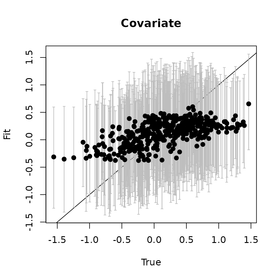
As with the fitted values, we see the predicted values seem to capture the pattern in the true estimates.
           used  (Mb) gc trigger  (Mb) max used  (Mb)
Ncells  2480422 132.5    4585492 244.9  4585492 244.9
Vcells 17913442 136.7   48759749 372.1 50621557 386.3
Spatially varying coefficient multi-season occupancy model
Consider the case where detection-nondetection data are collected
across multiple seasons (e.g., years, breeding periods) during which the
true occupancy status can change. Such spatio-temporal data can be used
to understand occurrence trends over time (e.g., Isaac et al. (2014)), as well as the
environmental variables that drive spatio-temporal shifts in species
distributions (e.g., Rushing et al.
(2020)). As an extension to the SVC occupancy model, here we
present a SVC multi-season occupancy model that estimates spatially
varying effects (as described previously) of covariates and accounts for
temporal autocorrelation using temporal random effects. This model is an
extension of the multi-season spatial (stPGOcc()) and
non-spatial (tPGOcc()) occupancy models introduced in
spOccupancy v0.4.0. See the vignette
on multiseason models for additional background information on
modeling spatio-temporal patterns in occupancy.
Basic model description
Let \(y_{k, t}(\boldsymbol{s}_j)\) denote the detection or nondetection of the species of interest at site \(j\) during replicate survey \(k\) during time period \(t\), with \(t = 1, \dots, T\). We model \(y_{k, t}(\boldsymbol{s}_j)\) conditional on the true occupancy status, \(z_t(\boldsymbol{s}_j)\) of the species at site \(j\) during time \(t\) according to
\[\begin{equation}\label{zTime} z_{t}(\boldsymbol{s}_j) \sim \text{Bernoulli}(\psi_t(\boldsymbol{s}_j)), \end{equation}\]
where \(\psi_t(\boldsymbol{s}_j)\) is the occurrence probability at site \(j\) during primary time period \(t\). We model \(\psi_{t}(\boldsymbol{s}_j)\) following
\[\begin{equation}\label{psiTime} \text{logit}(\psi_t(\boldsymbol{s}_j)) = \textbf{x}_t(\boldsymbol{s}_j)\boldsymbol{\beta} + \tilde{\textbf{x}}_t(\boldsymbol{s}_j)\textbf{w}(\boldsymbol{s}_j) + \eta_t, \end{equation}\]
where \(\eta_t\) is a random temporal effect and the other parameters are defined as before. Note that the covariates can now vary across space and/or time period. Because we assume the non-spatial (\(\boldsymbol{\beta})\) and spatially varying (\(\textbf{w}(\boldsymbol{s}_j)\)) coefficients are constant over the \(T\) primary time periods, they represent the average covariate effects across the temporal extent of the data. We model \(\eta_t\) as either an unstructured random effect (i.e., \(\eta_t \sim \text{Normal}(0, \sigma^2_{T})\)) or using a first-order autoregressive (i.e., AR(1)) covariance structure in which we estimate a temporal variance parameter, \(\sigma^2_T\), and a temporal correlation parameter, \(\rho\).
The data \(y_{k, t}(\boldsymbol{s}_j)\) are modeled conditional on the true occupancy status \(z_t(\boldsymbol{s}_j)\) analogous to the SVC occupancy model, with detection probability now allowed to vary across site, replicates, and/or primary time periods.
Simulating data with simTOcc()
The function simTOcc() simulates single-species
multi-season detection-nondetection data. simTOcc() has the
following arguments, which again closely resemble all other data
simulation functions in spOccupancy.
simTOcc(J.x, J.y, n.time, n.rep, n.rep.max, beta, alpha, sp.only = 0, trend = TRUE,
        psi.RE = list(), p.RE = list(), sp = FALSE, svc.cols = 1, cov.model,
        sigma.sq, phi, nu, ar1 = FALSE, rho, sigma.sq.t, x.positive = FALSE,
        mis.spec.type = 'none', scale.param = 1, avail, ...)
J.x and J.y indicate the number of spatial
locations to simulate data along a horizontal and vertical axis,
respectively, such that J.x * J.y is the total number of
sites (i.e., J). n.time indicates the number
of time periods over which data are collected. n.rep is a
numeric matrix with rows corresponding to sites and columns
corresponding to time periods where each element corresponds to the
number of replicate surveys performed within a given time period at a
given site (denoted as K in the previous model
description). Note that throughout we will refer to “time period” as the
additional temporal replication in multi-season models (often called
primary time period) and will use the term “replicate” to refer to the
multiple visits obtained at a given site during a given time period
(often called secondary time periods). n.rep.max is an
optional value that can be used to specify the maximum number of
replicate surveys, which is useful for emulating data from autonomous
monitoring approaches (e.g., camera traps) where sampling occurs over a
set number of time periods (e.g., days), but any individual site was not
sampled across all the time periods. beta and
alpha are numeric vectors containing the intercept and any
regression coefficient parameters for the occurrence and detection
portions of the occupancy model, respectively. sp.only is a
numeric vector specifying which occurrence covariates should only vary
over space and not over time. trend is a logical value
indicating whether or not a trend parameter is included in the model
(the trend is assumed to be the second covariate listed in
beta). psi.RE and p.RE are lists
that are used to specify random intercepts on occurrence and detection,
respectively, which are analogous to previous data simulation functions.
sp is a logical value indicating whether to simulate data
with at least one spatial Gaussian process for either the intercept or
some of the occupancy covariate effects. svc.cols is a
numeric vector indicating which of the covariates (including the
intercept) are generated with spatially varying effects.
cov.model specifies the covariance function used to model
the spatial dependence structure. Finally, sigma.sq is the
spatial variance parameter, phi is the spatial decay
parameter, and nu is the spatial smoothness parameter (only
applicable when cov.model = 'matern'). Note that
sigma.sq, phi, and nu should have
the same length as the number of spatially varying effects specified in
svc.cols. The x.positive argument indicates
whether or not the occupancy covariates should be simulated to be only
positive from a Uniform(0, 1) distribution (TRUE) or both
positive and negative and simulated from a Normal(0, 1) distribution
(FALSE). The arguments mis.spec.type and
scale.param are arguments that can be used to simulate
detection-nondetection data where the model is misspecified, while the
avail parameter can be used to simulate
detection-nondetection data where there is an availability component in
the model. See the manual page for simTOcc() for more
details on these last three arguments, which we will not address in this
vignette.
For this simulation, we will attempt to estimate a spatially varying
trend parameter. Such an analysis can provide useful information for
monitoring programs by allowing for prioritization of locations where
occupancy trends are declining. Additionally, it can often help generate
hypotheses as to what factors are driving the heterogenous trends across
space. Below we simulate data across 400 sites and ten time periods with
anywhere between 1-4 replicates at a given time-period, a spatially
varying intercept, a spatially varying trend on occupancy, and a single
covariate effect on detection. Note that we vary the number of time
periods each site is sampled. We assume both the occupancy intercept and
the trend vary across space, so we set svc.cols = c(1, 2).
We use an exponential correlation function. We do not include any
unstructured random effects on occurrence or detection.
set.seed(10)
J.x <- 20
J.y <- 20
# Total number of sites
(J <- J.x * J.y)
[1] 400
# Total number of time periods at each site
n.time <- sample(10, J, replace = TRUE)
n.time.max <- max(n.time)
# Number of replicates at each site/time period combination
n.rep <- matrix(NA, J, max(n.time))
for (j in 1:J) {
  n.rep[j, 1:n.time[j]] <- sample(4, n.time[j], replace = TRUE)
}
sp.only <- 0
# Simulate a trend parameter
trend <- TRUE
# Intercept and trend on occurrence
beta <- c(-0.5, -0.2)
# Intercept and covariate effect on detection
alpha <- c(0.9, -0.3)
# No unstructured random intercept on occurrence
psi.RE <- list()
# No unstructured random intercept on detection
p.RE <- list()
# Spatial decay for intercept and trend
phi <- c(3 / .8, 3 / .7)
# Spatial variance for intercept and trend
sigma.sq <- c(1, 0.5)
# Simulate data with an AR1 temporal process
ar1 <- TRUE
# Temporal variance of AR1 random effect
sigma.sq.t <- 0.5
# Temporal correlation of AR1 random effect
rho <- 0.25
# Simulate the occupancy covariate from a Normal(0, 1) distribution
x.positive <- FALSE
# Spatially varying coefficient columns
svc.cols <- c(1, 2)
# Simulate the data
dat <- simTOcc(J.x = J.x, J.y = J.y, n.time = n.time, n.rep = n.rep, beta = beta,
               alpha = alpha, sp.only = sp.only, trend = trend,
               psi.RE = psi.RE, p.RE = p.RE, sp = TRUE,
               sigma.sq = sigma.sq, phi = phi,
               cov.model = 'exponential', svc.cols = svc.cols,
               x.positive = x.positive, ar1 = ar1, sigma.sq.t = sigma.sq.t,
               rho = rho)
First let’s take a look at the true occupancy values averaged across all spatial locations to see if there appears to be an overall trend over time
str(dat)List of 15
$ X : num [1:400, 1:10, 1:2] 1 1 1 1 1 1 1 1 1 1 ...
$ X.p : num [1:400, 1:10, 1:4, 1:2] 1 1 1 1 1 1 1 1 1 1 ...
$ coords : num [1:400, 1:2] 0 0.0526 0.1053 0.1579 0.2105 ...
..- attr(*, "dimnames")=List of 2
.. ..$ : chr [1:400] "1" "2" "3" "4" ...
.. ..$ : NULL
$ coords.full: num [1:400, 1:2] 0 0.0526 0.1053 0.1579 0.2105 ...
..- attr(*, "dimnames")=List of 2
.. ..$ : NULL
.. ..$ : chr [1:2] "Var1" "Var2"
$ psi : num [1:400, 1:10] 0.992 0.984 0.934 0.679 0.722 ...
$ z : int [1:400, 1:10] 1 1 1 0 1 1 0 1 1 1 ...
$ p : num [1:400, 1:10, 1:4] 0.643 NA 0.685 0.586 0.713 ...
$ y : int [1:400, 1:10, 1:4] 1 NA 1 0 1 1 NA NA NA 1 ...
$ w : num [1:400, 1:2] 0.744 0.915 1.207 1.367 0.918 ...
$ w.grid : num [1:400, 1:2] 0.744 0.915 1.207 1.367 0.918 ...
$ X.p.re : logi NA
$ X.re : logi NA
$ alpha.star : logi NA
$ beta.star : logi NA
$ eta : num [1:10, 1] 1.068 -0.754 1.386 -0.101 -0.579 ...
# Plot average occupancy probability
plot(apply(dat$psi, 2, mean), pch = 19, xlab = 'Time Period',
     ylab = 'Average Occupancy Probability',
     cex = 1.5, frame = FALSE, ylim = c(0, 1))
The simulated data object consists of the same objects as we saw
previously with simOcc(). However, because of the
additional time period dimension, all of the objects (except for spatial
coordinates and spatially varying effects) now have an additional
dimension of time period. For example, the occurrence design matrix
X is now a three-dimensional array with dimensions
corresponding to site, time period, and covariate. We see on average
occupancy is decreasing over the simulated ten year period, which makes
sense given the average value we used to simulate the data (-0.2).
Below we extract the data we need to fit the model and create a plot of the spatially varying trend across the study region
# Detection-nondetection data
y <- dat$y
# Occurrence design matrix for fixed effects
X <- dat$X
# Detection design matrix for fixed effets
X.p <- dat$X.p
# Occurrence values
psi <- dat$psi
# Spatial coordinates
coords <- dat$coords
# Spatially varying intercept and covariate effects
w <- dat$w

cov.effect <- beta[2] + w[, 2]
plot.dat <- data.frame(x = coords[, 1],
                       y = coords[, 2],
                       cov.effect = cov.effect)
ggplot(plot.dat, aes(x = x, y = y, fill = cov.effect)) +
  geom_raster() +
  scale_fill_gradient2(midpoint = 0, low = '#B2182B', mid = 'white',
                       high = '#2166AC', na.value = NA) +
  theme_bw()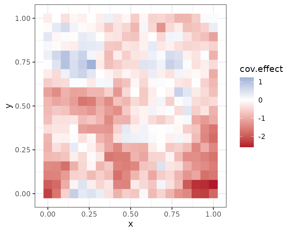
We see heterogenous trends across the study area with some locations showing a large decrease in occurrence (red) and others showing a large increase (blue).
We finally package up the data into the data list format for
multi-season occupancy models. As before, we will fit the model with 75%
of the spatial locations and then predict at the remaining 25% of the
locations. With multi-season occupancy models, the occurrence covariates
can now vary across both space and time, and so we specify
occ.covs as a list rather than as a matrix/data frame as we
saw with svcPGOcc(). See the
multi-season occupancy model vignette for additional details.
# Subset data for prediction.
# Split into fitting and prediction data set
pred.indx <- sample(1:J, round(J * .25), replace = FALSE)
y.fit <- y[-pred.indx, , ]
y.pred <- y[pred.indx, , ]
X.fit <- X[-pred.indx, , ]
X.pred <- X[pred.indx, , ]
X.p.fit <- X.p[-pred.indx, , , ]
X.p.pred <- X.p[pred.indx, , , ]
coords.fit <- coords[-pred.indx, ]
coords.pred <- coords[pred.indx, ]
psi.fit <- psi[-pred.indx, ]
psi.pred <- psi[pred.indx, ]
w.fit <- w[-pred.indx, ]
w.pred <- w[pred.indx, ]

# Package all data into a list
# Occurrence covariates
occ.covs <- list(trend = X.fit[, , 2])
# Detection covariates
det.covs <- list(det.cov.1 = X.p.fit[, , , 2])
# Package into a list for spOccupancy
data.list <- list(y = y.fit,
                  occ.covs = occ.covs,
                  det.covs = det.covs,
                  coords = coords.fit)
# Take a look at the data structure.
str(data.list)
List of 4
$ y : int [1:300, 1:10, 1:4] NA 1 0 1 NA NA 1 1 0 0 ...
$ occ.covs:List of 1
..$ trend: num [1:300, 1:10] -1.57 -1.57 -1.57 -1.57 -1.57 ...
$ det.covs:List of 1
..$ det.cov.1: num [1:300, 1:10, 1:4] NA 0.408 1.848 -1.321 NA ...
$ coords : num [1:300, 1:2] 0.0526 0.1053 0.1579 0.2632 0.3158 ...
..- attr(*, "dimnames")=List of 2
.. ..$ : chr [1:300] "2" "3" "4" "6" ...
.. ..$ : NULLFitting spatially varying coefficient multi-season occupancy models
with svcPGOcc()
The function svcTPGOcc() fits spatially-varyig
coefficients multi-season occupancy models. It’s arguments are exactly
identical to svcPGOcc(), with the only addition being the
ar1 argument.
svcTPGOcc(occ.formula, det.formula, data, inits, priors,
          tuning, svc.cols = 1, cov.model = 'exponential', NNGP = TRUE,
          n.neighbors = 15, search.type = 'cb', n.batch,
          batch.length, accept.rate = 0.43, n.omp.threads = 1,
          verbose = TRUE, ar1 = FALSE, n.report = 100,
          n.burn = round(.10 * n.batch * batch.length),
          n.thin = 1, n.chains = 1, k.fold, k.fold.threads = 1,
          k.fold.seed = 100, k.fold.only = FALSE, ...)
Given the similarity in the syntax for svcTPGOcc() and
svcPGOcc(), we won’t go into all that much detail on them
here. For additional details on the input parameters related to the
temporal parameters, see the multi-season
occupancy model vignette.
The occ.formula and det.formula are
specified in the same manner as we saw previously. The data
argument contains the list of the formatted data, which we discussed in
the preceding section for multi-season models.
data <- data.list
str(data)
List of 4
$ y : int [1:300, 1:10, 1:4] NA 1 0 1 NA NA 1 1 0 0 ...
$ occ.covs:List of 1
..$ trend: num [1:300, 1:10] -1.57 -1.57 -1.57 -1.57 -1.57 ...
$ det.covs:List of 1
..$ det.cov.1: num [1:300, 1:10, 1:4] NA 0.408 1.848 -1.321 NA ...
$ coords : num [1:300, 1:2] 0.0526 0.1053 0.1579 0.2632 0.3158 ...
..- attr(*, "dimnames")=List of 2
.. ..$ : chr [1:300] "2" "3" "4" "6" ...
.. ..$ : NULL
occ.formula <- ~ trend
det.formula <- ~ det.cov.1
Next we specify the initial values for all model parameters. We will
fit the model with an AR(1) temporal covariance structure, which
includes two additional parameters: sigma.sq.t (a temporal
variance parameter) and rho (a temporal correlation
parameter). We specifiy initial values for z to 1 if the species was
ever observed at the given site/time period combination and 0
otherwise.
z.inits <- apply(data$y, c(1, 2), function(a) as.numeric(sum(a, na.rm = TRUE) > 0))
inits <- list(beta = 0, alpha = 0, z = z.inits,
              sigma.sq = 1, phi = 3 / 0.5,
              sigma.sq.t = 1.5, rho = 0.2)
We specify priors in the priors argument just as we saw
with svcPGOcc(). We use an inverse-Gamma prior for the
temporal variance sigma.sq.t and a uniform prior for the
temporal correlation parameter rho.
priors <- list(beta.normal = list(mean = 0, var = 2.72),
               alpha.normal = list(mean = 0, var = 2.72),
               sigma.sq.t.ig = c(2, 0.5),
               rho.unif = c(-1, 1),
               sigma.sq.ig = list(a = 2, b = 1),
               phi.unif = list(a = 3 / 1, b = 3 / .1))
Next we specify parameters associated with the spatial random
effects. In particular, we set cov.model = 'exponential' to
use an exponential spatial correlation function,
n.neighbors = 5 to use an NNGP with 5 nearest neighbors,
and svc.cols = c(1, 2) to specify a spatially varying
intercept and trend. We also specify the ar1 argument to
indicate we will use an AR(1) temporal covariance structure.
cov.model <- 'exponential'
svc.cols <- c(1, 2)
n.neighbors <- 5
ar1 <- TRUE
Finally, we set the number of MCMC batches, batch length, the amount of burn-in, and our thinning rate.
n.batch <- 600
batch.length <- 25
# Total number of samples
n.batch * batch.length
[1] 15000
n.burn <- 10000
n.thin <- 20
We now run the model with svcTPGOcc() and take a look at
a summary of the results using summary().
# Approx. run time: ~ 0.5 min
out.svc.trend <- svcTPGOcc(occ.formula = occ.formula,
                           det.formula = det.formula,
                           data = data,
                           inits = inits,
                           priors = priors,
                           cov.model = cov.model,
                           svc.cols = svc.cols,
                           n.neighbors = n.neighbors,
                           n.batch = n.batch,
                           batch.length = batch.length,
                           verbose = TRUE,
                           ar1 = ar1,
                           n.report = 200,
                           n.burn = n.burn,
                           n.thin = n.thin,
                           n.chains = 1)
----------------------------------------
Preparing the data
----------------------------------------
----------------------------------------
Building the neighbor list
----------------------------------------
----------------------------------------
Building the neighbors of neighbors list
----------------------------------------
----------------------------------------
Model description
----------------------------------------
Spatial NNGP Multi-season Occupancy Model with Polya-Gamma latent
variable fit with 300 sites and 10 years.
Samples per chain: 15000 (600 batches of length 25)
Burn-in: 10000
Thinning Rate: 20
Number of Chains: 1
Total Posterior Samples: 250
Number of spatially-varying coefficients: 2
Using the exponential spatial correlation model.
Using 5 nearest neighbors.
Using an AR(1) temporal autocorrelation matrix.
Source compiled with OpenMP support and model fit using 1 thread(s).
Adaptive Metropolis with target acceptance rate: 43.0
----------------------------------------
Chain 1
----------------------------------------
Sampling ...
Batch: 200 of 600, 33.33%
Coefficient Parameter Acceptance Tuning
1 phi 24.0 0.84366
2 phi 64.0 0.70469
1 rho 40.0 1.05127
-------------------------------------------------
Batch: 400 of 600, 66.67%
Coefficient Parameter Acceptance Tuning
1 phi 36.0 0.87810
2 phi 32.0 0.81058
1 rho 48.0 1.11628
-------------------------------------------------
Batch: 600 of 600, 100.00%
summary(out.svc.trend)
Call:
svcTPGOcc(occ.formula = occ.formula, det.formula = det.formula,
    data = data, inits = inits, priors = priors, svc.cols = svc.cols,
    cov.model = cov.model, n.neighbors = n.neighbors, n.batch = n.batch,
    batch.length = batch.length, verbose = TRUE, ar1 = ar1, n.report = 200,
    n.burn = n.burn, n.thin = n.thin, n.chains = 1)

Samples per Chain: 15000
Burn-in: 10000
Thinning Rate: 20
Number of Chains: 1
Total Posterior Samples: 250
Run Time (min): 0.6035

Occurrence (logit scale):
               Mean     SD    2.5%     50%   97.5% Rhat ESS
(Intercept) -0.4663 0.3781 -1.2376 -0.4483  0.2023   NA  43
trend       -1.0250 0.2403 -1.5266 -1.0145 -0.5502   NA  82

Detection (logit scale):
               Mean     SD    2.5%     50%   97.5% Rhat ESS
(Intercept)  0.8863 0.0621  0.7645  0.8899  1.0076   NA 250
det.cov.1   -0.2638 0.0548 -0.3650 -0.2697 -0.1609   NA 300

Spatio-temporal Covariance:
                        Mean     SD    2.5%     50%   97.5% Rhat ESS
sigma.sq-(Intercept)  1.1699 0.3626  0.6351  1.1191  1.9350   NA  85
sigma.sq-trend        0.3085 0.1397  0.1422  0.2718  0.6384   NA  73
phi-(Intercept)       5.1202 1.4590  3.1189  4.8139  8.5697   NA  63
phi-trend            11.0315 7.6012  3.0406  8.5505 27.1412   NA  14
sigma.sq.t            0.4323 0.2205  0.1606  0.3782  1.0687   NA 250
rho                  -0.1995 0.2351 -0.6110 -0.2159  0.2818   NA 193
# Compare estimates to true values
beta
[1] -0.5 -0.2
alpha[1] 0.9 -0.3
sigma.sq[1] 1.0 0.5
phi[1] 3.750000 4.285714
rho[1] 0.25
sigma.sq.t[1] 0.5Next, we extract the full SVC values using the
getSVCSamples() function and then compare the estimated
values to those used to generate the model.
# Intercept ---------------------------------------------------------------
svc.samples <- getSVCSamples(out.svc.trend)
int.quants <- apply(svc.samples[["(Intercept)"]], 2, quantile,
                    probs = c(0.025, 0.5, 0.975))
svc.true.fit <- beta + w.fit
plot(svc.true.fit[, 1], int.quants[2, ], pch = 19,
     ylim = c(min(int.quants[1, ]), max(int.quants[3, ])),
     xlab = "True", ylab = "Fit", main = 'Intercept')
abline(0, 1)
arrows(svc.true.fit[, 1], int.quants[2, ], svc.true.fit[, 1], col = 'gray',
       int.quants[1, ], length = 0.02, angle = 90)
arrows(svc.true.fit[, 1], int.quants[1, ], svc.true.fit[, 1], col = 'gray',
       int.quants[3, ], length = 0.02, angle = 90)
points(svc.true.fit[, 1], int.quants[2, ], pch = 19)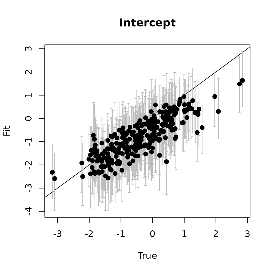
# Trend -------------------------------------------------------------------
trend.quants <- apply(svc.samples[["trend"]], 2, quantile,
                      probs = c(0.025, 0.5, 0.975))
plot(svc.true.fit[, 2], trend.quants[2, ], pch = 19,
     ylim = c(min(trend.quants[1, ]), max(trend.quants[3, ])),
     xlab = "True", ylab = "Fit", main = 'Spatially-Varying Trends')
abline(0, 1)
arrows(svc.true.fit[, 2], trend.quants[2, ], svc.true.fit[, 2], col = 'gray',
       trend.quants[1, ], length = 0.02, angle = 90)
arrows(svc.true.fit[, 2], trend.quants[1, ], svc.true.fit[, 2], col = 'gray',
       trend.quants[3, ], length = 0.02, angle = 90)
points(svc.true.fit[, 2], trend.quants[2, ], pch = 19)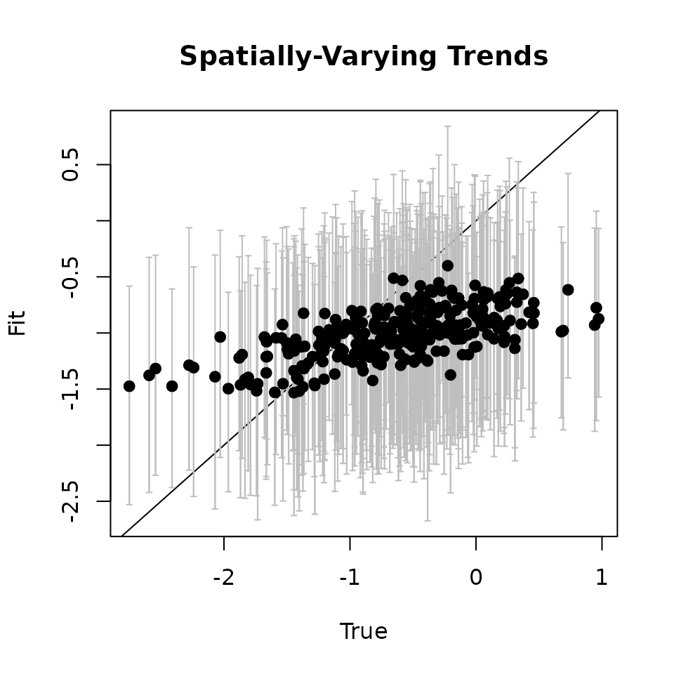
We see our model does a good job of recovering the true parameter values for both the spatially varying intercept and spatially varying trend.
Posterior Predictive Checks
Next we run a posterior predictive check using a Freeman-Tukey statistic and grouping by site.
ppc.out <- ppcOcc(out.svc.trend, fit.stat = 'freeman-tukey', group = 1)Currently on time period 1 out of 10Currently on time period 2 out of 10Currently on time period 3 out of 10Currently on time period 4 out of 10Currently on time period 5 out of 10Currently on time period 6 out of 10Currently on time period 7 out of 10Currently on time period 8 out of 10Currently on time period 9 out of 10Currently on time period 10 out of 10
summary(ppc.out)
Call:
ppcOcc(object = out.svc.trend, fit.stat = "freeman-tukey", group = 1)

Samples per Chain: 15000
Burn-in: 10000
Thinning Rate: 20
Number of Chains: 1
Total Posterior Samples: 250

----------------------------------------
    All time periods combined
----------------------------------------
Bayesian p-value:  0.52

----------------------------------------
    Individual time periods
----------------------------------------
Time Period 1 Bayesian p-value: 0.5
Time Period 2 Bayesian p-value: 0.424
Time Period 3 Bayesian p-value: 0.404
Time Period 4 Bayesian p-value: 0.58
Time Period 5 Bayesian p-value: 0.596
Time Period 6 Bayesian p-value: 0.516
Time Period 7 Bayesian p-value: 0.368
Time Period 8 Bayesian p-value: 0.48
Time Period 9 Bayesian p-value: 0.656
Time Period 10 Bayesian p-value: 0.676
Fit statistic:  freeman-tukey
As expected, we see all Bayesian p-values are quite close to the optimal 0.5.
Model Comparison using WAIC
Here we use WAIC to compare to a model that assumes the temporal
trend is constant over space using the stPGOcc() function
(or equivalently, we could use svcTPGOcc() with
svc.cols = 1).
priors.stPGOcc <- list(beta.normal = priors$beta.normal,
                       alpha.normal = priors$alpha.normal,
                       sigma.sq.t.ig = priors$sigma.sq.t.ig,
                       rho.unif = priors$rho.unif,
                       phi.unif = c(3 / 1, 3 / 0.1),
                       sigma.sq.ig = c(2, 1))
out.stPGOcc <- stPGOcc(occ.formula = occ.formula,
                       det.formula = det.formula,
                       data = data,
                       inits = inits,
                       priors = priors.stPGOcc,
                       cov.model = cov.model,
                       n.neighbors = n.neighbors,
                       n.batch = n.batch,
                       batch.length = batch.length,
                       verbose = TRUE,
                       ar1 = ar1,
                       n.report = 200,
                       n.burn = n.burn,
                       n.thin = n.thin,
                       n.chains = 1)
----------------------------------------
Preparing the data
----------------------------------------
----------------------------------------
Building the neighbor list
----------------------------------------
----------------------------------------
Building the neighbors of neighbors list
----------------------------------------
----------------------------------------
Model description
----------------------------------------
Spatial NNGP Multi-season Occupancy Model with Polya-Gamma latent
variable fit with 300 sites and 10 primary time periods.
Samples per chain: 15000 (600 batches of length 25)
Burn-in: 10000
Thinning Rate: 20
Number of Chains: 1
Total Posterior Samples: 250
Using the exponential spatial correlation model.
Using 5 nearest neighbors.
Using an AR(1) temporal autocorrelation matrix.
Source compiled with OpenMP support and model fit using 1 thread(s).
Adaptive Metropolis with target acceptance rate: 43.0
----------------------------------------
Chain 1
----------------------------------------
Sampling ...
Batch: 200 of 600, 33.33%
Parameter Acceptance Tuning
phi 16.0 0.77880
rho 48.0 1.23368
-------------------------------------------------
Batch: 400 of 600, 66.67%
Parameter Acceptance Tuning
phi 72.0 0.86071
rho 40.0 1.20925
-------------------------------------------------
Batch: 600 of 600, 100.00%
# SVC multi-season occupancy model
waicOcc(out.svc.trend)
elpd pD WAIC
-1752.7337 105.1898 3715.8469
# Spatial multi-season occupancy model
waicOcc(out.stPGOcc)
elpd pD WAIC
-1783.99835 75.68679 3719.37027 The lower WAIC value lends support for the model with the spatially varying trend compared to a model where the trend is assumed constant over space.
Prediction
Finally, we can use the predict() function to predict
relative occurrence and the effects of the covariates at new (and old)
locations. The t.cols argument specifies the time periods
over which you want to generate predictions. Here we will predict
occupancy at the hold out locations for all ten time periods.
# Take a look at X.pred, the design matrix for the prediction locations
head(X.pred)
, , 1
[,1] [,2] [,3] [,4] [,5] [,6] [,7] [,8] [,9] [,10]
[1,] 1 1 1 1 1 1 1 1 1 1
[2,] 1 1 1 1 1 1 1 1 1 1
[3,] 1 1 1 1 1 1 1 1 1 1
[4,] 1 1 1 1 1 1 1 1 1 1
[5,] 1 1 1 1 1 1 1 1 1 1
[6,] 1 1 1 1 1 1 1 1 1 1
, , 2
[,1] [,2] [,3] [,4] [,5] [,6] [,7]
[1,] -1.566503 -1.218391 -0.8702795 -0.5221677 -0.1740559 0.1740559 0.5221677
[2,] -1.566503 -1.218391 -0.8702795 -0.5221677 -0.1740559 0.1740559 0.5221677
[3,] -1.566503 -1.218391 -0.8702795 -0.5221677 -0.1740559 0.1740559 0.5221677
[4,] -1.566503 -1.218391 -0.8702795 -0.5221677 -0.1740559 0.1740559 0.5221677
[5,] -1.566503 -1.218391 -0.8702795 -0.5221677 -0.1740559 0.1740559 0.5221677
[6,] -1.566503 -1.218391 -0.8702795 -0.5221677 -0.1740559 0.1740559 0.5221677
[,8] [,9] [,10]
[1,] 0.8702795 1.218391 1.566503
[2,] 0.8702795 1.218391 1.566503
[3,] 0.8702795 1.218391 1.566503
[4,] 0.8702795 1.218391 1.566503
[5,] 0.8702795 1.218391 1.566503
[6,] 0.8702795 1.218391 1.566503
# Predict occupancy at the 400 new sites
out.pred <- predict(out.svc.trend, X.pred, coords.pred, t.cols = 1:n.time.max)
----------------------------------------
Prediction description
----------------------------------------
Spatial NNGP Multi-season Occupancy model with Polya-Gamma latent
variable fit with 300 observations and 10 years.
Number of fixed covariates 2 (including intercept if specified).
Using the exponential spatial correlation model.
Using 5 nearest neighbors.
Number of MCMC samples 250.
Predicting at 100 non-sampled locations.
Source compiled with OpenMP support and model fit using 1 threads.
-------------------------------------------------
Predicting
-------------------------------------------------
Location: 100 of 100, 100.00%
Generating latent occupancy state
# Use the getSVCSamples() function to extract the SVC values
# at the prediction locations
svc.pred.samples <- getSVCSamples(out.svc.trend, pred.object = out.pred)
# True covariate effect values at new locations
trend.pred <- beta[2] + w.pred[, 2]
# Get meian and 95% CIs of the SVC for the trendariate effect
trend.pred.quants <- apply(svc.pred.samples[["trend"]], 2, quantile,
                           probs = c(0.025, 0.5, 0.975))
plot(trend.pred, trend.pred.quants[2, ], pch = 19,
     ylim = c(min(trend.pred.quants[1, ]), max(trend.pred.quants[3, ])),
     xlab = "True", ylab = "Fit", main = 'Spatially varying trend')
abline(0, 1)
arrows(trend.pred, trend.pred.quants[2, ], trend.pred, col = 'gray',
       trend.pred.quants[1, ], length = 0.02, angle = 90)
arrows(trend.pred, trend.pred.quants[1, ], trend.pred, col = 'gray',
       trend.pred.quants[3, ], length = 0.02, angle = 90)
points(trend.pred, trend.pred.quants[2, ], pch = 19)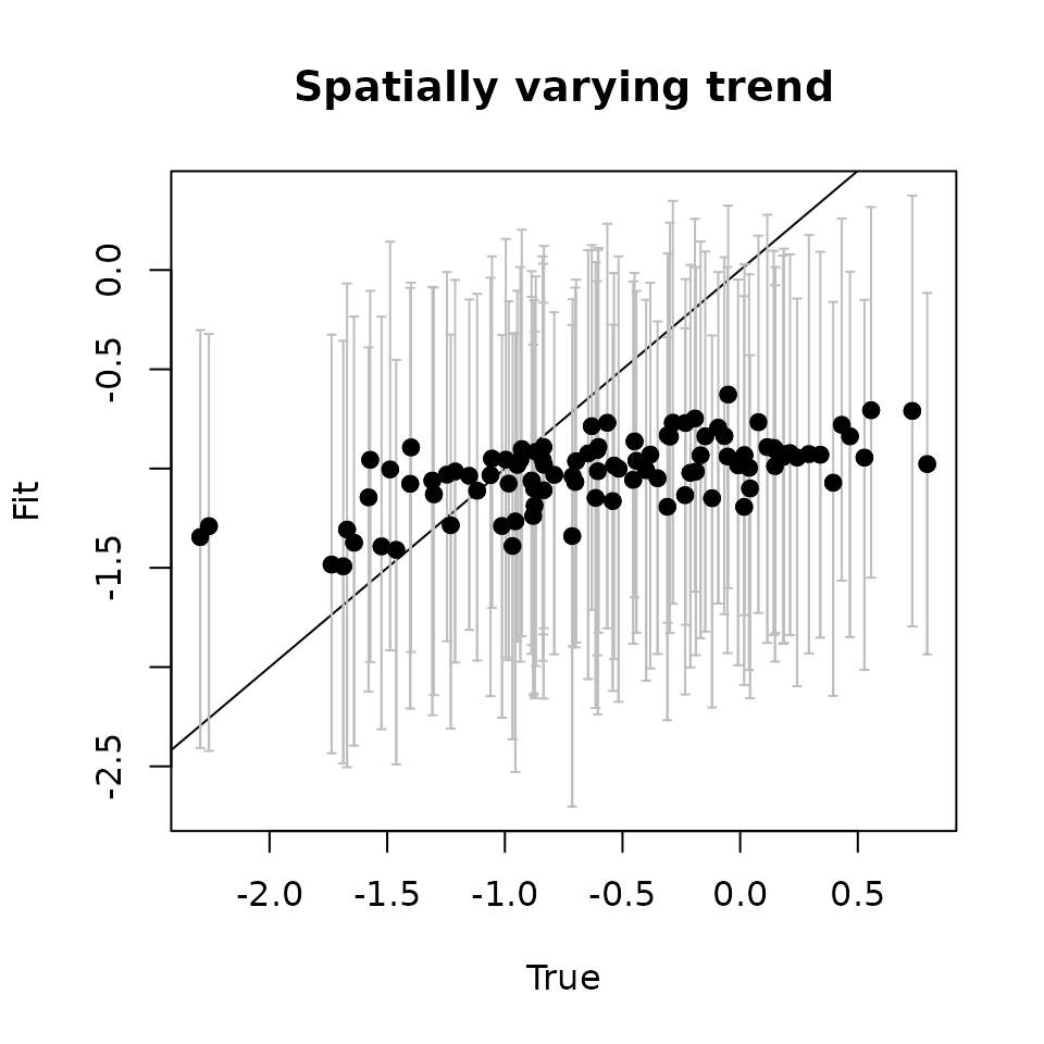
           used  (Mb) gc trigger  (Mb) max used  (Mb)
Ncells  2664338 142.3    4585492 244.9  4585492 244.9
Vcells 17722517 135.3   48759749 372.1 50621557 386.3
Spatially varying coefficient multi-season generalized linear model
Basic model description
To model spatio-temporal patterns in occurrence when ignoring imperfect detection, we directly model the detection-nondetection data analogous to the SVC GLM, with all data and parameters now varying over time. The occurrence status of the species at site \(j\) during primary time period \(t\) (\(\psi_t(\boldsymbol{s}_j)\)) is analogous to the SVC multi-season occupancy model.
Simulating data with simTBinom()
The function simTBinom() simulates single-species
multi-season detection-nondetection data assuming perfect detection.
simTBinom() has the following arguments, which again
closely resemble all other data simulation functions in
spOccupancy.
simTBinom(J.x, J.y, n.time, weights, beta, sp.only = 0,
          trend = TRUE, psi.RE = list(), sp = FALSE,
          cov.model, sigma.sq, phi, nu, svc.cols = 1,
          ar1 = FALSE, rho, sigma.sq.t, x.positive = FALSE, ...)
All parameters are the same as those described previously for
simTBinom() and simTOcc(). Below we simulate
data from 400 sites over 10 years, with uneven sampling over the 10
years across the sites. As with the SVC multi-season occupancy model,
our goal for this simulation is to assess a spatially varying trend.
set.seed(500)
J.x <- 20
J.y <- 20
# Total number of sites
(J <- J.x * J.y)
[1] 400
# Total number of time periods at each site
n.time <- sample(10, J, replace = TRUE)
n.time.max <- max(n.time)
# Number of Binomial replicates at each site/time period combination.
weights <- matrix(NA, J, max(n.time))
for (j in 1:J) {
  weights[j, 1:n.time[j]] <- sample(4, n.time[j], replace = TRUE)
}
sp.only <- 0
# Simulate a trend parameter
trend <- TRUE
# Intercept and trend on relative occurrence
beta <- c(-0.5, -0.2)
# No unstructured random intercept on relative occurrence
psi.RE <- list()
# Spatial decay for intercept and trend
phi <- c(3 / .8, 3 / .7)
# Spatial variance for intercept and trend
sigma.sq <- c(1, 0.5)
# Simulate data with an AR1 temporal process
ar1 <- TRUE
# Temporal variance of AR1 random effect
sigma.sq.t <- 0.5
# Temporal correlation of AR1 random effect
rho <- 0.25
# Spatially varying coefficient columns
svc.cols <- c(1, 2)
# Simulate the data
dat <- simTBinom(J.x = J.x, J.y = J.y, n.time = n.time, weights = weights,
                 beta = beta, sp.only = sp.only, trend = trend, psi.RE = psi.RE,
                 sp = TRUE, sigma.sq = sigma.sq, phi = phi,
                 cov.model = 'exponential', svc.cols = svc.cols,
                 ar1 = ar1, sigma.sq.t = sigma.sq.t, rho = rho)
str(dat)
List of 8
$ X : num [1:400, 1:10, 1:2] 1 1 1 1 1 1 1 1 1 1 ...
$ coords : num [1:400, 1:2] 0 0.0526 0.1053 0.1579 0.2105 ...
..- attr(*, "dimnames")=List of 2
.. ..$ : NULL
.. ..$ : chr [1:2] "Var1" "Var2"
$ psi : num [1:400, 1:10] 0.25286 0.06884 0.0829 0.03187 0.00752 ...
$ y : int [1:400, 1:10] 2 0 1 0 0 0 0 0 0 0 ...
$ w : num [1:400, 1:2] -1.246 -1.52 -1.033 -0.798 -1.627 ...
$ X.re : logi NA
$ beta.star: logi NA
$ eta : num [1:10, 1] -0.3429 0.0803 -0.5192 -0.1028 -0.0615 ...
# Plot average occupancy probability
plot(apply(dat$psi, 2, mean), pch = 19, xlab = 'Time Period',
     ylab = 'Average Occupancy Probability',
     cex = 1.5, frame = FALSE, ylim = c(0, 1))
We see a small decline in relative occurrence probability over the simulated ten years.
Below we extract the data we need to fit the model and create a plot of the spatially varying trend across the study region
# Detection-nondetection data
y <- dat$y
# Design matrix for fixed effects
X <- dat$X
# Occurrence values
psi <- dat$psi
# Spatial coordinates
coords <- dat$coords
# Spatially varying intercept and covariate effects
w <- dat$w

trend <- beta[2] + w[, 2]
plot.dat <- data.frame(x = coords[, 1],
                       y = coords[, 2],
                       trend = trend)
ggplot(plot.dat, aes(x = x, y = y, fill = trend)) +
  geom_raster() +
  scale_fill_gradient2(midpoint = 0, low = '#B2182B', mid = 'white', high = '#2166AC',
                       na.value = NA) +
  theme_bw() +
  labs(x = 'Easting', y = 'Northing', fill = 'Trend')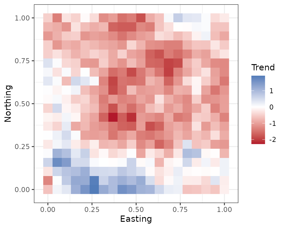
Lastly, we package up the data in a list required for fitting the
multi-season spatially varying coefficient GLM. We create a list with
the following objects: y (the detection-nondetection data
specified as a two-dimensional matrix), covs (the
covariates specified as a list), weights (a matrix of
binomial weights indicating the number of Bernoulli trials), and
coords (a matrix of spatial coordinates). As before, we
subset the data for prediction to only fit the model with 75% of the
sites.
# Subset data for prediction.
# Split into fitting and prediction data set
pred.indx <- sample(1:J, round(J * .25), replace = FALSE)
y.fit <- y[-pred.indx, ]
y.pred <- y[pred.indx, ]
X.fit <- X[-pred.indx, , ]
X.pred <- X[pred.indx, , ]
coords.fit <- coords[-pred.indx, ]
coords.pred <- coords[pred.indx, ]
psi.fit <- psi[-pred.indx, ]
psi.pred <- psi[pred.indx, ]
w.fit <- w[-pred.indx, ]
w.pred <- w[pred.indx, ]
weights.fit <- weights[-pred.indx, ]
weights.pred <- weights[pred.indx, ]

# Package all data into a list
# Occurrence covariates
covs <- list(trend = X.fit[, , 2])
# Package into a list for spOccupancy
data.list <- list(y = y.fit,
                  covs = covs,
                  weights = weights.fit,
                  coords = coords.fit)
# Take a look at the data structure.
str(data.list)
List of 4
$ y : int [1:300, 1:10] 2 0 1 0 0 0 0 0 0 0 ...
$ covs :List of 1
..$ trend: num [1:300, 1:10] -1.57 -1.57 -1.57 -1.57 -1.57 ...
$ weights: int [1:300, 1:10] 4 1 1 3 4 3 4 3 2 3 ...
$ coords : num [1:300, 1:2] 0 0.0526 0.1053 0.1579 0.2105 ...
..- attr(*, "dimnames")=List of 2
.. ..$ : NULL
.. ..$ : chr [1:2] "Var1" "Var2"Fitting spatially varying coefficient generalized linear models with
svcTPGBinom()
The function svcTPGBinom() fits spatially-varyig
coefficient multi-season generalized linear models.
svcTPGBinom(formula, data, inits, priors,
            tuning, svc.cols = 1, cov.model = 'exponential', NNGP = TRUE,
            n.neighbors = 15, search.type = 'cb', n.batch,
            batch.length, accept.rate = 0.43, n.omp.threads = 1,
            verbose = TRUE, ar1 = FALSE, n.report = 100,
            n.burn = round(.10 * n.batch * batch.length),
            n.thin = 1, n.chains = 1, k.fold, k.fold.threads = 1,
            k.fold.seed = 100, k.fold.only = FALSE, ...)
There are no new arguments or details for fitting models with
svcTPGBinom(), so we will go ahead and fit the model after
specifying all the model arguments.
# Formatted data list
data <- data.list
str(data)
List of 4
$ y : int [1:300, 1:10] 2 0 1 0 0 0 0 0 0 0 ...
$ covs :List of 1
..$ trend: num [1:300, 1:10] -1.57 -1.57 -1.57 -1.57 -1.57 ...
$ weights: int [1:300, 1:10] 4 1 1 3 4 3 4 3 2 3 ...
$ coords : num [1:300, 1:2] 0 0.0526 0.1053 0.1579 0.2105 ...
..- attr(*, "dimnames")=List of 2
.. ..$ : NULL
.. ..$ : chr [1:2] "Var1" "Var2"
# Model formula
formula <- ~ trend
# Initial values
inits <- list(beta = 0, sigma.sq = 1, phi = 3 / 0.5,
              sigma.sq.t = 1.5, rho = 0.2)
# Priors
priors <- list(beta.normal = list(mean = 0, var = 2.72),
               sigma.sq.t.ig = c(2, 0.5),
               rho.unif = c(-1, 1),
               sigma.sq.ig = list(a = 2, b = 1),
               phi.unif = list(a = 3 / 1, b = 3 / .1))
# Exponential covariance function
cov.model <- 'exponential'
# Spatially varying intercept and trend
svc.cols <- c(1, 2)
# Fit model with a NNGP with 5 neighbors
n.neighbors <- 5
# Include an AR(1) temporal covariance structure.
ar1 <- TRUE
# MCMC parameters
n.batch <- 600
batch.length <- 25
# Total number of samples
n.batch * batch.length
[1] 15000
n.burn <- 10000
n.thin <- 20
# Approx. run time: ~ 0.5 min
out.svc.trend <- svcTPGBinom(formula = formula,
                             data = data,
                             inits = inits,
                             priors = priors,
                             cov.model = cov.model,
                             svc.cols = svc.cols,
                             n.neighbors = n.neighbors,
                             n.batch = n.batch,
                             batch.length = batch.length,
                             verbose = TRUE,
                             ar1 = ar1,
                             n.report = 200,
                             n.burn = n.burn,
                             n.thin = n.thin,
                             n.chains = 1)
----------------------------------------
Preparing the data
----------------------------------------
----------------------------------------
Building the neighbor list
----------------------------------------
----------------------------------------
Building the neighbors of neighbors list
----------------------------------------
----------------------------------------
Model description
----------------------------------------
Spatial NNGP Multi-season Binomial Model with Polya-Gamma latent
variable fit with 300 sites and 10 years.
Samples per chain: 15000 (600 batches of length 25)
Burn-in: 10000
Thinning Rate: 20
Number of Chains: 1
Total Posterior Samples: 250
Number of spatially-varying coefficients: 2
Using the exponential spatial correlation model.
Using 5 nearest neighbors.
Using an AR(1) temporal autocorrelation matrix.
Source compiled with OpenMP support and model fit using 1 thread(s).
Adaptive Metropolis with target acceptance rate: 43.0
----------------------------------------
Chain 1
----------------------------------------
Sampling ...
Batch: 200 of 600, 33.33%
Coefficient Parameter Acceptance Tuning
1 phi 28.0 0.58860
2 phi 60.0 0.70469
1 rho 32.0 1.28403
-------------------------------------------------
Batch: 400 of 600, 66.67%
Coefficient Parameter Acceptance Tuning
1 phi 40.0 0.53259
2 phi 40.0 0.81058
1 rho 28.0 1.30996
-------------------------------------------------
Batch: 600 of 600, 100.00%
summary(out.svc.trend)
Call:
svcTPGBinom(formula = formula, data = data, inits = inits, priors = priors,
    svc.cols = svc.cols, cov.model = cov.model, n.neighbors = n.neighbors,
    n.batch = n.batch, batch.length = batch.length, verbose = TRUE,
    ar1 = ar1, n.report = 200, n.burn = n.burn, n.thin = n.thin,
    n.chains = 1)

Samples per Chain: 15000
Burn-in: 10000
Thinning Rate: 20
Number of Chains: 1
Total Posterior Samples: 250
Run Time (min): 0.5436

Occurrence (logit scale):
               Mean     SD    2.5%    50%  97.5% Rhat ESS
(Intercept) -0.1490 0.2990 -0.7855 -0.131 0.4739   NA  32
trend       -0.2644 0.3101 -0.7975 -0.279 0.3572   NA  20

Spatio-temporal Covariance:
                        Mean     SD    2.5%     50%   97.5% Rhat ESS
sigma.sq-(Intercept)  0.7342 0.1810  0.4590  0.7109  1.1274   NA 141
sigma.sq-trend        0.7398 0.2080  0.4181  0.7101  1.1573   NA 120
phi-(Intercept)       7.6085 2.4949  3.7415  7.2722 13.0823   NA 160
phi-trend             5.0191 1.4382  3.0930  4.7755  8.6837   NA  81
sigma.sq.t            0.2524 0.1365  0.0930  0.2154  0.6464   NA 250
rho                  -0.0135 0.2508 -0.5345 -0.0059  0.4355   NA 250
# Compare estimates to true values
beta
[1] -0.5 -0.2
alpha[1] 0.9 -0.3
sigma.sq[1] 1.0 0.5
phi[1] 3.750000 4.285714
rho[1] 0.25
sigma.sq.t[1] 0.5Let’s extract the spatially varying intercept and spatially varying
trend estimates from our model using getSVCSamples() and
compare them to the true values.
# Intercept ---------------------------------------------------------------
svc.samples <- getSVCSamples(out.svc.trend)
int.quants <- apply(svc.samples[["(Intercept)"]], 2, quantile,
                    probs = c(0.025, 0.5, 0.975))
svc.true.fit <- beta + w.fit
plot(svc.true.fit[, 1], int.quants[2, ], pch = 19,
     ylim = c(min(int.quants[1, ]), max(int.quants[3, ])),
     xlab = "True", ylab = "Fit", main = 'Intercept')
abline(0, 1)
arrows(svc.true.fit[, 1], int.quants[2, ], svc.true.fit[, 1], col = 'gray',
       int.quants[1, ], length = 0.02, angle = 90)
arrows(svc.true.fit[, 1], int.quants[1, ], svc.true.fit[, 1], col = 'gray',
       int.quants[3, ], length = 0.02, angle = 90)
points(svc.true.fit[, 1], int.quants[2, ], pch = 19)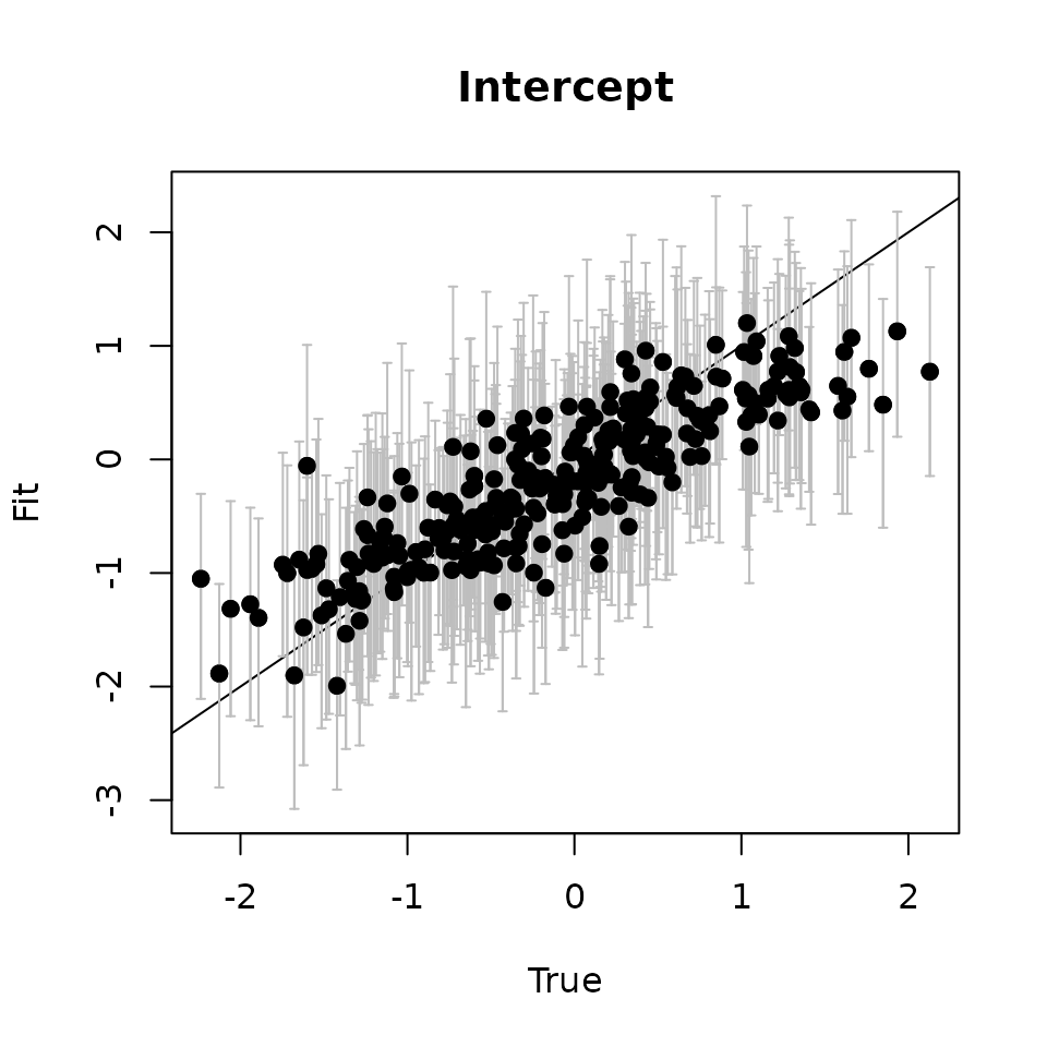
# Trend -------------------------------------------------------------------
trend.quants <- apply(svc.samples[["trend"]], 2, quantile,
                      probs = c(0.025, 0.5, 0.975))
plot(svc.true.fit[, 2], trend.quants[2, ], pch = 19,
     ylim = c(min(trend.quants[1, ]), max(trend.quants[3, ])),
     xlab = "True", ylab = "Fit", main = 'Spatially-Varying Trends')
abline(0, 1)
arrows(svc.true.fit[, 2], trend.quants[2, ], svc.true.fit[, 2], col = 'gray',
       trend.quants[1, ], length = 0.02, angle = 90)
arrows(svc.true.fit[, 2], trend.quants[1, ], svc.true.fit[, 2], col = 'gray',
       trend.quants[3, ], length = 0.02, angle = 90)
points(svc.true.fit[, 2], trend.quants[2, ], pch = 19)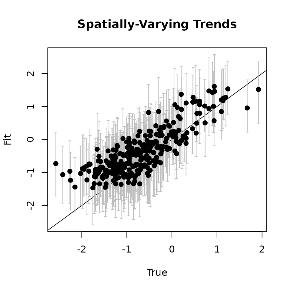
We see our model does a good job of recovering the true parameter values for both the spatially varying intercept and spatially varying trend.
Model Comparison using WAIC
Here we use WAIC to compare our full SVC model to a model that
assumes the temporal trend is constant over space by setting
svc.cols = 1.
out.trend.const <- svcTPGBinom(formula = formula,
                               data = data,
                               inits = inits,
                               priors = priors,
                               svc.cols = 1,
                               cov.model = cov.model,
                               n.neighbors = n.neighbors,
                               n.batch = n.batch,
                               batch.length = batch.length,
                               verbose = TRUE,
                               ar1 = ar1,
                               n.report = 200,
                               n.burn = n.burn,
                               n.thin = n.thin,
                               n.chains = 1)
----------------------------------------
Preparing the data
----------------------------------------
----------------------------------------
Building the neighbor list
----------------------------------------
----------------------------------------
Building the neighbors of neighbors list
----------------------------------------
----------------------------------------
Model description
----------------------------------------
Spatial NNGP Multi-season Binomial Model with Polya-Gamma latent
variable fit with 300 sites and 10 years.
Samples per chain: 15000 (600 batches of length 25)
Burn-in: 10000
Thinning Rate: 20
Number of Chains: 1
Total Posterior Samples: 250
Number of spatially-varying coefficients: 1
Using the exponential spatial correlation model.
Using 5 nearest neighbors.
Using an AR(1) temporal autocorrelation matrix.
Source compiled with OpenMP support and model fit using 1 thread(s).
Adaptive Metropolis with target acceptance rate: 43.0
----------------------------------------
Chain 1
----------------------------------------
Sampling ...
Batch: 200 of 600, 33.33%
Coefficient Parameter Acceptance Tuning
1 phi 48.0 0.58860
1 rho 36.0 1.18530
-------------------------------------------------
Batch: 400 of 600, 66.67%
Coefficient Parameter Acceptance Tuning
1 phi 44.0 0.58860
1 rho 36.0 1.30996
-------------------------------------------------
Batch: 600 of 600, 100.00%
# SVC multi-season GLM
waicOcc(out.svc.trend)
elpd pD WAIC
-1517.713 198.032 3431.490
# Spatial multi-season GLM
waicOcc(out.trend.const)
elpd pD WAIC
-1674.1340 162.3747 3673.0174 Prediction
Finally, we use the predict() function to predict
relative occurrence and the effects of the covariates at new (and old)
locations over the simulated ten tme periods.
# Take a look at X.pred, the design matrix for the prediction locations
head(X.pred)
, , 1
[,1] [,2] [,3] [,4] [,5] [,6] [,7] [,8] [,9] [,10]
[1,] 1 1 1 1 1 1 1 1 1 1
[2,] 1 1 1 1 1 1 1 1 1 1
[3,] 1 1 1 1 1 1 1 1 1 1
[4,] 1 1 1 1 1 1 1 1 1 1
[5,] 1 1 1 1 1 1 1 1 1 1
[6,] 1 1 1 1 1 1 1 1 1 1
, , 2
[,1] [,2] [,3] [,4] [,5] [,6] [,7]
[1,] -1.566503 -1.218391 -0.8702795 -0.5221677 -0.1740559 0.1740559 0.5221677
[2,] -1.566503 -1.218391 -0.8702795 -0.5221677 -0.1740559 0.1740559 0.5221677
[3,] -1.566503 -1.218391 -0.8702795 -0.5221677 -0.1740559 0.1740559 0.5221677
[4,] -1.566503 -1.218391 -0.8702795 -0.5221677 -0.1740559 0.1740559 0.5221677
[5,] -1.566503 -1.218391 -0.8702795 -0.5221677 -0.1740559 0.1740559 0.5221677
[6,] -1.566503 -1.218391 -0.8702795 -0.5221677 -0.1740559 0.1740559 0.5221677
[,8] [,9] [,10]
[1,] 0.8702795 1.218391 1.566503
[2,] 0.8702795 1.218391 1.566503
[3,] 0.8702795 1.218391 1.566503
[4,] 0.8702795 1.218391 1.566503
[5,] 0.8702795 1.218391 1.566503
[6,] 0.8702795 1.218391 1.566503
# Predict occupancy at the 400 new sites
out.pred <- predict(out.svc.trend, X.pred, coords.pred, t.cols = 1:n.time.max,
                    weights = weights.pred)
----------------------------------------
Prediction description
----------------------------------------
Spatial NNGP Multi-season Occupancy model with Polya-Gamma latent
variable fit with 300 observations and 10 years.
Number of fixed covariates 2 (including intercept if specified).
Using the exponential spatial correlation model.
Using 5 nearest neighbors.
Number of MCMC samples 250.
Predicting at 100 non-sampled locations.
Source compiled with OpenMP support and model fit using 1 threads.
-------------------------------------------------
Predicting
-------------------------------------------------
Location: 100 of 100, 100.00%
Generating latent occupancy state
# Use the getSVCSamples() function to extract the SVC values
# at the prediction locations
svc.pred.samples <- getSVCSamples(out.svc.trend, pred.object = out.pred)
# True covariate effect values at new locations
trend.pred <- beta[2] + w.pred[, 2]
# Get meian and 95% CIs of the SVC for the trendariate effect
trend.pred.quants <- apply(svc.pred.samples[["trend"]], 2, quantile,
                           probs = c(0.025, 0.5, 0.975))
plot(trend.pred, trend.pred.quants[2, ], pch = 19,
     ylim = c(min(trend.pred.quants[1, ]), max(trend.pred.quants[3, ])),
     xlab = "True", ylab = "Fit", main = 'Spatially varying trend')
abline(0, 1)
arrows(trend.pred, trend.pred.quants[2, ], trend.pred, col = 'gray',
       trend.pred.quants[1, ], length = 0.02, angle = 90)
arrows(trend.pred, trend.pred.quants[1, ], trend.pred, col = 'gray',
       trend.pred.quants[3, ], length = 0.02, angle = 90)
points(trend.pred, trend.pred.quants[2, ], pch = 19)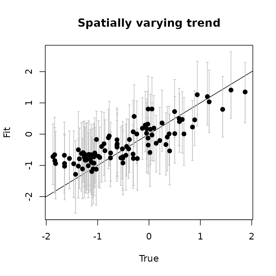
           used  (Mb) gc trigger  (Mb) max used  (Mb)
Ncells  2681336 143.2    4585492 244.9  4585492 244.9
Vcells 20074273 153.2   48759749 372.1 50621557 386.3
Multi-species spatially varying coefficient occupancy models
Now consider the case where there are multiple species of interest, \(N\), that are observed during data collection. We seek to jointly model the occupancy of the \(N\) species in a single model that accommodates residual correlations between species and allows for sharing of information across species via random effects. Such multi-species approaches often have improved precision and accuracy of estimates compared to single-species models (Clark et al. 2014; Zipkin et al. 2010).
Basic model description
Using similar notation to the single-species models, we model the true presence-absence state of species \(i\) at site \(\boldsymbol{s}_j\) following
\[\begin{equation}\label{zMS} z_i(\boldsymbol{s}_j) \sim \text{Bernoulli}(\psi_i(\boldsymbol{s}_j) z^\ast_i(\boldsymbol{s}_j)), \end{equation}\]
where \(\psi_i(\boldsymbol{s}_j)\) is the occupancy probability of species \(i\) at site \(j\), and \(z^\ast_i(\boldsymbol{s}_j)\) is a binary auxiliary data source indicating whether site \(j\) is within the range of species \(i\). Such data can be obtained from a variety of sources, including international databases (e.g., BirdLife International, IUCN), field guides, or expert opinion. We suggest buffering the auxiliary data range map by a suitable distance to account for potential inaccuracies in the auxiliary data. Inclusion of such auxiliary range data can drastically reduce the run time of the model if certain species can only exist at a subset of all the spatial locations in the data set (Socolar et al. 2022). If auxiliary range data are not available, \(z^\ast_i(\boldsymbol{s}_j)\) can be removed (or equivalently, \(z^\ast_i(\boldsymbol{s}_j) = 1\) for all \(j\)).
At sites within a species’ range, we model species-specific occupancy probability as
\[\begin{equation}\label{psiMS} \text{logit}(\psi_i(\boldsymbol{s}_j)) = \textbf{x}(\boldsymbol{s}_j)\boldsymbol{\beta}_i + \tilde{\textbf{x}}(\boldsymbol{s}_j)\textbf{w}_i^\ast(\boldsymbol{s}_j), \end{equation}\]
with all parameters as defined before, but now spatial and non-spatial effects are unique to each species. We assume the same variables have spatially-varying effects (or not) for all species although relaxing this assumption is a focus of some of our ongoing work. We model the non-spatial component of the \(h\)th regression coefficient for each species \(i\) hierarchically from a common community-level distribution to share information across species . More specifically, we have
\[\begin{equation}\label{betaMS} \beta_{i, h} \sim \text{Normal}(\mu_{\beta_h}, \tau^2_{\beta_h}), \end{equation}\] where \(\mu_{\beta_h}\) is the average non-spatial effect across all species in the community, and \(\tau^2_{\beta_h}\) is the variability in the non-spatial effect across all species.
We seek to jointly model the species-specific spatial effects, \(\textbf{w}^\ast_{i, h}\), to account for correlation in species-specific responses to covariate effects, as well as residual correlations between species after accounting for their relationships with any covariates included in the model. We use a spatial factor model (Hogan and Tchernis 2004), a dimension reduction technique that accounts for correlations in species-specific responses, while drastically reducing computational run time compared to other common alternatives. Here, we decompose \(\text{w}^\ast_{i, h}(\boldsymbol{s}_j)\) into a linear combination of \(q\) latent factors and their associated species-specific coefficients (i.e., factor loadings). Thus for each SVC in the model, we have
\[\begin{equation}\label{wStar} \text{w}^\ast_{i, h}(\boldsymbol{s}_j) = \boldsymbol{\lambda}^\top_{i, h}\textbf{w}_{h}(\boldsymbol{s}_j), \end{equation}\] where \(\boldsymbol{\lambda}_{i, h}^\top\) is the \(i\)th row of factor loadings from the \(N \times q\) loadings matrix \(\boldsymbol{\Lambda}_h\), and \(\textbf{w}_h(\boldsymbol{s}_j)\) is a \(q \times 1\) vector of independent spatial factors at site \(j\). As in the single-species SVC occupancy model, we model each of the \(r = 1, \dots, q\) spatial factors for each of the \(\tilde{H}\) spatially-varying effects with an NNGP.
Analogous to the single-species case, we model the observed detection-nondetection of each species \(i\) at site \(j\) during replicate survey \(k\), \(y_{i, k}(\boldsymbol{s}_j)\) conditional on the true presence-absence of each species, \(z_{i}(\boldsymbol{s}_j)\), following the single-species equations, with all parameters now varying by species. We model the species-specific detection regression coefficients (\(\boldsymbol{\alpha}_i\)) hierarchically, analogous to the non-spatial occupancy regression coefficients.
We assume Gaussian priors for all mean parameters and inverse-Gamma priors for variance parameters. Additional restrictions on the factors loadings matrix \(\boldsymbol{\Lambda}_h\) for each spatially-varying coefficient \(h\) are required to ensure identifiability (Taylor-Rodriguez et al. 2019; Doser, Finley, and Banerjee 2023). We fix all elements in the upper triangle to 0 and set the diagonal elements to 1. We additionally fix the spatial variance parameters \(\sigma^2_h\) of each latent spatial process to 1. We assign standard Gaussian priors for the lower triangular elements in \(\boldsymbol{\Lambda}\) and assign each spatial decay parameter \(\phi_{r, h}\) an independent uniform prior. For full statistical details on these models, see Doser, Finley, and Banerjee (2023) and Doser et al. (2024).
Simulating data with simMsOcc()
The function simMsOcc() simulates multi-species
detection-nondetection data. simMsOcc() has the following
arguments, which should look familiar to other simulation functions in
spOccupancy.
simMsOcc(J.x, J.y, n.rep, n.rep.max, N, beta, alpha, psi.RE = list(),
         p.RE = list(), sp = FALSE, svc.cols = 1, cov.model,
         sigma.sq, phi, nu, factor.model = FALSE, n.factors,
         range.probs, ...)
J.x and J.y indicate the number of spatial
locations to simulate data along a horizontal and vertical axis,
respectively, such that J.x * J.y is the total number of
sites (i.e., \(J\)). n.rep
is a numeric vector of length J that indicates the number
of replicates at each site of the \(J\)
sites (denoted as \(K\) in model
notation). n.rep.max is an optional single numeric value
that indicates the maximum number of replicate surveys, which can be
useful to simulate data from something like a camera trap protocol where
the replicates are “days” (or some other unit of time), but any one
individual site is not sampled for all days. N is the
number of species to simulate. beta and alpha
are matrices containing the intercept and any regression coefficient
parameters for the occurrence and detection portions of the occupancy
model for each species, respectively, for each species. The rows of the
matrix correspond to species and columns correspond to parameter.
psi.RE and p.RE are lists used to specify
random intercepts on detection and occurrence, which follow the same
format as single-species models. sp, svc.cols,
and cov.model are arguments that control whether data are
simulated with spatial random effects and/or spatially varying
coefficients. The argument factor.model is a logical value,
indicating whether a factor model is used to simulate the spatial random
effects. This should be set to TRUE for simulating
multi-species spatially-varying coefficient occupancy models. The
argument n.factors is a numeric value that indicates the
number of factors to use to simulate the species-specific
spatially-varying coefficients. sigma.sq, phi,
and nu are numeric vectors, each with
n.factors * length(svc.cols) values for the spatial
variance, spatial decay, and spatial smoothness parameters,
respectively, that control the spatially varying coefficients. Note the
spatial smoothness parameter is only relevant when
cov.model = 'matern'. Lastly, the range.probs
argument is a numeric vector with N values (one for each
species), where each value should fall between 0 and 1. Each value
indicates the probability that one of the \(J\) spatial locations in the simulated data
set falls within the simulated range of the species. By default, this is
set to 1, which means each spatial location is within the range of every
species in the data set.
Below we simulate data from 6 species across 400 locations with 3
replicates at a given site, a single covariate effect on occurrence, and
a single covariate effect on detection. We assume both the occupancy
intercept and the effect of the covariate vary across space, so we set
svc.cols = c(1, 2). We use an exponential correlation
function, and don’t include any unstructured random intercepts. We then
plot the spatially-varying effect of the covariate across the region for
the first two species in the data set. We will use two spatial factors
for both the intercept and spatially varying coefficient.
set.seed(300)
J.x <- 20
J.y <- 20
J <- J.x * J.y
n.rep <- rep(3, J)
N <- 6
# Community-level covariate effects
# Occurrence
beta.mean <- c(0.2, 0)
p.occ <- length(beta.mean)
tau.sq.beta <- c(0.6, 0.5)
# Detection
alpha.mean <- c(0, 0.5)
tau.sq.alpha <- c(1, 0.5)
p.det <- length(alpha.mean)
# No random effects
psi.RE <- list()
p.RE <- list()
# Draw species-level effects from community means.
beta <- matrix(NA, nrow = N, ncol = p.occ)
alpha <- matrix(NA, nrow = N, ncol = p.det)
for (i in 1:p.occ) {
  beta[, i] <- rnorm(N, beta.mean[i], sqrt(tau.sq.beta[i]))
}
for (i in 1:p.det) {
  alpha[, i] <- rnorm(N, alpha.mean[i], sqrt(tau.sq.alpha[i]))
}
n.factors <- 2
svc.cols <- c(1, 2)
p.svc <- length(svc.cols)
q.p.svc <- n.factors * p.svc
alpha.true <- alpha
phi <- runif(q.p.svc, 3 / 0.9, 3 / 0.3)
# Assume each species' range spans the study area
range.probs <- runif(N, 1, 1)
factor.model <- TRUE
cov.model <- 'exponential'
sp <- TRUE

dat <- simMsOcc(J.x = J.x, J.y = J.y, n.rep = n.rep, N = N, beta = beta, alpha = alpha,
                psi.RE = psi.RE, p.RE = p.RE, phi = phi, sp = TRUE, svc.cols = svc.cols,
                cov.model = 'exponential', n.factors = n.factors, factor.model = TRUE,
                range.probs = range.probs)
str(dat)
List of 16
$ X : num [1:400, 1:2] 1 1 1 1 1 1 1 1 1 1 ...
$ X.p : num [1:400, 1:3, 1:2] 1 1 1 1 1 1 1 1 1 1 ...
$ coords : num [1:400, 1:2] 0 0.0526 0.1053 0.1579 0.2105 ...
..- attr(*, "dimnames")=List of 2
.. ..$ : chr [1:400] "1" "2" "3" "4" ...
.. ..$ : NULL
$ coords.full: num [1:400, 1:2] 0 0.0526 0.1053 0.1579 0.2105 ...
..- attr(*, "dimnames")=List of 2
.. ..$ : NULL
.. ..$ : chr [1:2] "Var1" "Var2"
$ w :List of 2
..$ : num [1:2, 1:400] 1.1109 0.1151 1.4692 0.0721 1.2278 ...
..$ : num [1:2, 1:400] -0.0923 1.6828 -0.7281 1.3397 -1.5559 ...
$ psi : num [1:6, 1:400] 0.923 0.898 0.85 0.772 0.83 ...
$ z : num [1:6, 1:400] 1 1 1 1 1 1 1 1 1 1 ...
$ p : num [1:6, 1:400, 1:3] 0.243 0.614 0.659 0.642 0.835 ...
$ y : int [1:6, 1:400, 1:3] 0 1 1 0 1 0 0 0 1 0 ...
$ X.p.re : logi NA
$ X.re : logi NA
$ alpha.star : logi NA
$ beta.star : logi NA
$ lambda :List of 2
..$ : num [1:6, 1:2] 1 0.6618 0.2351 -0.0672 0.0764 ...
..$ : num [1:6, 1:2] 1 -0.0579 0.015 0.1641 -1.3651 ...
$ X.w : num [1:400, 1:2] 1 1 1 1 1 1 1 1 1 1 ...
$ range.ind : int [1:6, 1:400] 1 1 1 1 1 1 1 1 1 1 ...
# Detection-nondetection data
y <- dat$y
# Occurrence design matrix for fixed effects
X <- dat$X
# Detection design matrix for fixed effets
X.p <- dat$X.p
# Occurrence values
psi <- dat$psi
# Spatial coordinates
coords <- dat$coords
# Spatially-varying intercept for each species
svi.true <- dat$lambda[[1]] %*% dat$w[[1]]
# Spatially-varying coefficient for covariate for each species
svc.true <- dat$lambda[[2]] %*% dat$w[[2]]
# Full SVC effect for each species (w + beta)
cov.effect <- svc.true + beta[, 2]
plot.dat <- data.frame(x = coords[, 1],
                       y = coords[, 2],
                       svc.sp.1 = cov.effect[1, ],
                       svc.sp.2 = cov.effect[2, ])
ggplot(plot.dat, aes(x = x, y = y, fill = svc.sp.1)) +
  geom_tile(col = 'black') +
  scale_fill_gradient2(midpoint = 0, low = '#B2182B', mid = 'white',
                       high = '#2166AC', na.value = NA) +
  theme_bw() +
  labs(title = 'Species 1 SVC')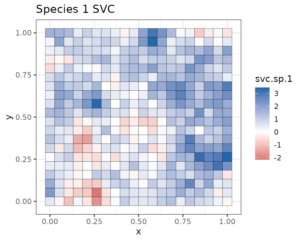
ggplot(plot.dat, aes(x = x, y = y, fill = svc.sp.2)) +
  geom_tile(col = 'black') +
  scale_fill_gradient2(midpoint = 0, low = '#B2182B', mid = 'white',
                       high = '#2166AC', na.value = NA) +
  theme_bw() +
  labs(title = 'Species 2 SVC')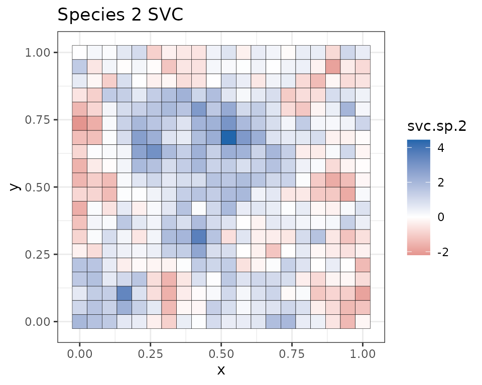
Notice we see clear differences in the effect of the covariate across
the two species and across space for each of the species. Next, we
package up the data into the data list format for multi-species
occupancy models. As before, we will fit the model with 75% of the
spatial locations and then predict at the remaining 25% of the
locations. Notice the range.ind component of the data list
specified below, which is a binary matrix indicating whether or not the
given site falls within the range of a given species. Here, we simulated
our data such that every site was within the range of each species, and
so this is just a matrix of 1s. This argument is not necessary to
specify in such a situation as this is also the default value, but here
we include it explicitly.
# Subset data for prediction.
# Split into fitting and prediction data set
pred.indx <- sample(1:J, round(J * .25), replace = FALSE)
y.fit <- y[, -pred.indx, ]
y.pred <- y[, pred.indx, ]
X.fit <- X[-pred.indx, ]
X.pred <- X[pred.indx, ]
X.p.fit <- X.p[-pred.indx, , ]
X.p.pred <- X.p[pred.indx, , ]
coords.fit <- coords[-pred.indx, ]
coords.pred <- coords[pred.indx, ]
psi.fit <- psi[, -pred.indx]
psi.pred <- psi[, pred.indx]
svc.true.fit <- svc.true[, -pred.indx]
svc.true.pred <- svc.true[, pred.indx]
svi.true.fit <- svi.true[, -pred.indx]
svi.true.pred <- svi.true[, pred.indx]
range.ind.fit <- dat$range.ind[, -pred.indx]

# Package all data into a list
# Occurrence covariates
occ.covs <- X.fit[, 2, drop = FALSE]
colnames(occ.covs) <- c('occ.cov.1')
# Detection covariates
det.covs <- list(det.cov.1 = X.p.fit[, , 2])
# Package into a list for spOccupancy
data.list <- list(y = y.fit,
                  occ.covs = occ.covs,
                  det.covs = det.covs,
                  coords = coords.fit,
                  range.ind = range.ind.fit)
# Take a look at the data structure.
str(data.list)
List of 5
$ y : int [1:6, 1:300, 1:3] 0 1 1 0 1 0 0 0 1 0 ...
$ occ.covs : num [1:300, 1] 0.2349 1.3387 -0.0994 1.0369 -0.3455 ...
..- attr(*, "dimnames")=List of 2
.. ..$ : NULL
.. ..$ : chr "occ.cov.1"
$ det.covs :List of 1
..$ det.cov.1: num [1:300, 1:3] 0.564 -0.724 1.952 -0.789 1.104 ...
$ coords : num [1:300, 1:2] 0 0.0526 0.1053 0.1579 0.2105 ...
..- attr(*, "dimnames")=List of 2
.. ..$ : chr [1:300] "1" "2" "3" "4" ...
.. ..$ : NULL
$ range.ind: int [1:6, 1:300] 1 1 1 1 1 1 1 1 1 1 ...Fitting multi-species spatially varying coefficient occupancy models
with svcMsPGOcc()
The function svcMsPGOcc() fits multi-species SVC
occupancy models. svcMsPGOcc() has the following
arguments:
svcMsPGOcc(occ.formula, det.formula, data, inits, priors, tuning,
           svc.cols = 1, cov.model = 'exponential', NNGP = TRUE,
           n.neighbors = 15, search.type = 'cb', std.by.sp = FALSE,
           n.factors, n.batch, batch.length,
           accept.rate = 0.43, n.omp.threads = 1,
           verbose = TRUE, n.report = 100,
           n.burn = round(.10 * n.batch * batch.length), n.thin = 1,
           n.chains = 1, ...)
The arguments are nearly identical to svcPGOcc(), with
the only exceptions being the std.by.sp and the
n.factors arguments. The argument std.by.sp is
a logical value indicating whether covariates should be standardized
individually for each species when the study area is larger than some
individual species’ range. In the case where auxiliary species range
information is not provided or all species ranges span the study area,
this argument will have no influence on the results. When auxiliary
range information is provided and species ranges vary across the modeled
area, setting std.by.sp = TRUE will separately standardize
(i.e., subtract the mean and divide by the standard deviation) all the
occurrence covariates using only the covariate values that fall within
that species’ range. We generally recommend doing this when modeling
species with different ranges, as it can help with convergence and
mixing of the MCMC chains, particularly when there are some species
whose range only occurs in one portion of the covariate space.
The n.factors argument is used to specify how many
factors one should use in the factor modeling approach for each SVC.
Choosing the number of factors is not always straightforward, and how
many factors can/should be used is dependent on the data at hand. We
present guidance on choosing the number of factors, among other things,
in a separate
vignette. Given the large similarities in syntax with
svcPGOcc(), we do not go into too much detail here on the
arguments. Here we set n.factors to 2, which is what we
used to simulate the data.
We will also mention that the prior on the spatial decay parameter
phi may be quite important in order to generate reasonable
results that don’t show extreme amounts of overfitting. This is not
specific to SVC models, but given the fact that SVC models have multiple
Gaussian processes (or rather NNGPs), there is a higher chance of
extreme overfitting occurring for specific data sets. In short, if you
fit a model and find large amounts of overfitting in the predicted
occurrence probabilities, then you may look into restricting the lower
bound of the effective spatial range (or equivalently, the upper bound
on the spatial decay parameter, \(\phi\)). This is discussed in much more
detail here.
You may also notice that there are no arguments related to
cross-validation for svcMsPGOcc(). This is not currently
implemented for multi-species SVC models. However, the GitHub
repositories associated with some of our recent work on SVC occupancy
models provide examples of how to do assessments of predictive
performance with multi-species SVC models.
Below we specify all the model arguments, including the priors, initial values, and tuning values. Default values of the initial values, priors, and tuning values are provided such that these arguments can be ignored, but for such complicated models like this, one may need to more carefully consider these values in order to yield adequate mixing/convergence of the MCMC chains. This is a common feature of Bayesian models, in that as models become more complicated, the more problems we may encounter when trying to fit them. Once we specify all the function arguments, we go ahead and fit the model.
# Occurrence formula
occ.formula <- ~ occ.cov.1
# Detection formula
det.formula <- ~ det.cov.1
# Specify which columns/parameters are modeled as SVCs
svc.cols <- c(1, 2)
# OR
# svc.cols <- c('(Intercept)', 'occ.cov.1')
# Exponential correlation function
cov.model <- 'exponential'
# Specify initial values
inits.list <- list(alpha.comm = 0, # Community-level detection mean parameters
                   beta.comm = 0, # Community-level occurrence mean parameters
                   beta = 0, # Species-level occurrence effects
                   alpha = 0, # Species-level detection effects
                   tau.sq.beta = 1, # Community-level occurrence variances
                   tau.sq.alpha = 1, # Community-level detection variances
                   phi = 3 / .5, # Spatial decay parameter
                   # Latent species-specific occurrence
                   z = apply(y.fit, c(1, 2), max, na.rm = TRUE))
# Specify prior values
prior.list <- list(beta.comm.normal = list(mean = 0, var = 2.72),
                   alpha.comm.normal = list(mean = 0, var = 2.72),
                   tau.sq.beta.ig = list(a = 0.1, b = 0.1),
                   tau.sq.alpha.ig = list(a = 0.1, b = 0.1),
                   phi.unif = list(a = 3 / 1, b = 3 / 0.1))
# Tuning list
tuning.list <- list(phi = 0.7)
# MCMC criteria
batch.length <- 25
n.batch <- 800
n.burn <- 10000
n.thin <- 10
n.chains <- 3
n.report <- 200
accept.rate <- 0.43
# NNGP criteria
n.omp.threads <- 1
NNGP <- TRUE
n.neighbors <- 5
# Specify the number of spatial factors to use
n.factors <- 2
# Fit the model (Approx. run time: 4 min)
out.ms <- svcMsPGOcc(occ.formula = occ.formula, det.formula = det.formula,
                     data = data.list, inits = inits.list,
                     priors = prior.list, tuning = tuning.list,
                     svc.cols = svc.cols, cov.model = cov.model, NNGP = NNGP,
                     n.neighbors = n.neighbors, n.factors = n.factors,
                     n.batch = n.batch, batch.length = batch.length,
                     accept.rate = accept.rate, n.omp.threads = n.omp.threads,
                     verbose = TRUE, n.report = n.report, n.burn = n.burn,
                     n.thin = n.thin, n.chains = n.chains)
----------------------------------------
Preparing to run the model
----------------------------------------lambda is not specified in initial values.
Setting initial values of the lower triangle to random values from a standard normalw is not specified in initial values.
Setting initial value to 0----------------------------------------
Building the neighbor list
----------------------------------------
----------------------------------------
Building the neighbors of neighbors list
----------------------------------------
----------------------------------------
Model description
----------------------------------------
Spatial Factor NNGP Multispecies Occupancy Model with Polya-Gamma latent
variable fit with 300 sites and 6 species.
Samples per chain: 20000 (800 batches of length 25)
Burn-in: 10000
Thinning Rate: 10
Number of Chains: 3
Total Posterior Samples: 3000
Number of spatially-varying coefficients: 2
Using the exponential spatial correlation model.
Using 2 latent spatial factors.
Using 5 nearest neighbors.
Source compiled with OpenMP support and model fit using 1 thread(s).
Adaptive Metropolis with target acceptance rate: 43.0
----------------------------------------
Chain 1
----------------------------------------
Sampling ...
Batch: 200 of 800, 25.00%
Coefficient Latent Factor Acceptance Tuning
1 1 24.0 1.48190
1 2 32.0 0.88102
2 1 40.0 0.91698
2 2 56.0 0.54516
-------------------------------------------------
Batch: 400 of 800, 50.00%
Coefficient Latent Factor Acceptance Tuning
1 1 28.0 1.51184
1 2 32.0 0.69303
2 1 12.0 1.26279
2 2 40.0 0.55617
-------------------------------------------------
Batch: 600 of 800, 75.00%
Coefficient Latent Factor Acceptance Tuning
1 1 20.0 1.57354
1 2 32.0 0.93550
2 1 48.0 1.23779
2 2 44.0 0.52378
-------------------------------------------------
Batch: 800 of 800, 100.00%
----------------------------------------
Chain 2
----------------------------------------
Sampling ...
Batch: 200 of 800, 25.00%
Coefficient Latent Factor Acceptance Tuning
1 1 36.0 1.21328
1 2 28.0 0.82971
2 1 52.0 1.07608
2 2 32.0 0.51341
-------------------------------------------------
Batch: 400 of 800, 50.00%
Coefficient Latent Factor Acceptance Tuning
1 1 40.0 1.45256
1 2 32.0 0.76592
2 1 36.0 1.05477
2 2 36.0 0.54516
-------------------------------------------------
Batch: 600 of 800, 75.00%
Coefficient Latent Factor Acceptance Tuning
1 1 16.0 1.36797
1 2 68.0 0.91698
2 1 16.0 0.82971
2 2 40.0 0.54516
-------------------------------------------------
Batch: 800 of 800, 100.00%
----------------------------------------
Chain 3
----------------------------------------
Sampling ...
Batch: 200 of 800, 25.00%
Coefficient Latent Factor Acceptance Tuning
1 1 64.0 1.45256
1 2 24.0 0.91698
2 1 56.0 0.97368
2 2 44.0 0.54516
-------------------------------------------------
Batch: 400 of 800, 50.00%
Coefficient Latent Factor Acceptance Tuning
1 1 44.0 1.39560
1 2 36.0 0.88102
2 1 44.0 1.26279
2 2 24.0 0.47394
-------------------------------------------------
Batch: 600 of 800, 75.00%
Coefficient Latent Factor Acceptance Tuning
1 1 68.0 1.63775
1 2 56.0 0.73589
2 1 20.0 1.09782
2 2 52.0 0.51341
-------------------------------------------------
Batch: 800 of 800, 100.00%
# Quick summary of model results
summary(out.ms)
Call:
svcMsPGOcc(occ.formula = occ.formula, det.formula = det.formula,
    data = data.list, inits = inits.list, priors = prior.list,
    tuning = tuning.list, svc.cols = svc.cols, cov.model = cov.model,
    NNGP = NNGP, n.neighbors = n.neighbors, n.factors = n.factors,
    n.batch = n.batch, batch.length = batch.length, accept.rate = accept.rate,
    n.omp.threads = n.omp.threads, verbose = TRUE, n.report = n.report,
    n.burn = n.burn, n.thin = n.thin, n.chains = n.chains)

Samples per Chain: 20000
Burn-in: 10000
Thinning Rate: 10
Number of Chains: 3
Total Posterior Samples: 3000
Run Time (min): 3.8701

----------------------------------------
    Community Level
----------------------------------------
Occurrence Means (logit scale):
              Mean     SD   2.5%    50%  97.5%   Rhat  ESS
(Intercept) 1.0984 0.3447 0.4311 1.0901 1.7947 1.0035 1904
occ.cov.1   0.8777 0.3715 0.1291 0.8775 1.6042 1.0066  619

Occurrence Variances (logit scale):
              Mean     SD   2.5%    50%  97.5%   Rhat  ESS
(Intercept) 0.6261 0.9469 0.0673 0.3708 2.6756 1.0331 1609
occ.cov.1   0.3991 0.5226 0.0533 0.2513 1.6266 1.0105 2514

Detection Means (logit scale):
               Mean     SD    2.5%     50%  97.5%   Rhat  ESS
(Intercept) -0.1365 0.4951 -1.0990 -0.1419 0.8727 1.0028 2905
det.cov.1    0.4751 0.1545  0.1793  0.4731 0.8005 1.0003 3000

Detection Variances (logit scale):
              Mean     SD   2.5%    50% 97.5%   Rhat  ESS
(Intercept) 1.6909 1.8675 0.4214 1.2316 5.458 1.0777 2962
det.cov.1   0.1468 0.1663 0.0332 0.1023 0.541 1.0107 3000

----------------------------------------
    Species Level
----------------------------------------
Occurrence (logit scale):
                  Mean     SD    2.5%    50%  97.5%   Rhat  ESS
(Intercept)-sp1 1.5245 0.4773  0.7520 1.4731 2.6403 1.0078  615
(Intercept)-sp2 1.3438 0.2987  0.7880 1.3332 1.9718 1.0277  653
(Intercept)-sp3 1.0135 0.2580  0.5505 0.9994 1.5951 1.0092 1258
(Intercept)-sp4 0.8221 0.2594  0.3580 0.8101 1.3920 1.0048 1769
(Intercept)-sp5 0.4501 0.2569 -0.0154 0.4366 1.0121 1.0034 1171
(Intercept)-sp6 1.7178 0.5998  0.8048 1.6265 3.1243 1.0183  567
occ.cov.1-sp1   1.3427 0.4318  0.5869 1.3158 2.2682 1.0172  779
occ.cov.1-sp2   0.3961 0.3186 -0.2344 0.3964 1.0239 1.0048  533
occ.cov.1-sp3   0.9855 0.3776  0.2924 0.9785 1.7914 1.0046  626
occ.cov.1-sp4   0.6892 0.4277 -0.1317 0.6794 1.5853 1.0005  399
occ.cov.1-sp5   1.1808 0.4243  0.3747 1.1698 2.0354 1.0084  525
occ.cov.1-sp6   0.7451 0.4657 -0.1586 0.7324 1.6877 1.0057  683

Detection (logit scale):
                   Mean     SD    2.5%     50%   97.5%   Rhat  ESS
(Intercept)-sp1 -1.1957 0.1260 -1.4353 -1.1922 -0.9409 1.0132 1546
(Intercept)-sp2  0.1539 0.0968 -0.0274  0.1513  0.3478 1.0021 2730
(Intercept)-sp3  0.5377 0.0974  0.3458  0.5376  0.7295 1.0040 3000
(Intercept)-sp4 -0.2184 0.1131 -0.4364 -0.2206  0.0054 1.0022 3000
(Intercept)-sp5  1.3469 0.1174  1.1150  1.3471  1.5745 1.0030 2265
(Intercept)-sp6 -1.3812 0.1377 -1.6456 -1.3848 -1.1162 1.0039  979
det.cov.1-sp1    0.3409 0.0900  0.1658  0.3423  0.5140 0.9999 3000
det.cov.1-sp2    0.5740 0.0867  0.4010  0.5725  0.7414 1.0015 3215
det.cov.1-sp3    0.2308 0.0863  0.0593  0.2315  0.4000 1.0007 3398
det.cov.1-sp4    0.8420 0.1054  0.6440  0.8401  1.0551 1.0037 2751
det.cov.1-sp5    0.3886 0.1067  0.1836  0.3878  0.5948 1.0025 3000
det.cov.1-sp6    0.4989 0.0962  0.3097  0.4956  0.6841 1.0009 3208

----------------------------------------
    Spatial Covariance
----------------------------------------
                     Mean     SD   2.5%     50%   97.5%   Rhat ESS
phi-1-(Intercept) 20.4765 7.3050 4.2193 22.3586 29.6375 1.0385 115
phi-2-(Intercept) 15.2877 7.7322 3.7565 14.8954 29.0557 1.1041 159
phi-1-occ.cov.1   18.3872 7.8054 3.6113 19.5716 29.4748 1.0482  90
phi-2-occ.cov.1   10.1241 4.0765 4.3040  9.5097 20.9554 1.0338 182
We generally see fairly adequate convergence of the model, with the
potential exception of some of the spatial decay parameters. For more
details on assessing convergence of spOccupancy model
objects, particularly of spatial factor models like this one, see this
vignette. Because we are using simulated data, we can compare the
estimates from our model to the true values we used to simulate the
data. Below we generate a couple very simple plots to compare the
species-specific occurrence and detection regression coefficient
estimates to the true values.
# Mean non-spatial occurrence regression coefficients
beta.means <- apply(out.ms$beta.samples, 2, mean)
# True values
beta.true <- beta
plot(beta.true, beta.means, pch = 19)
abline(0, 1)
# Mean detection regression coefficients
alpha.means <- apply(out.ms$alpha.samples, 2, mean)
# True values
alpha.true <- alpha
plot(alpha.true, alpha.means, pch = 19)
abline(0, 1)
As with single-species SVC models, we can use the
getSVCSamples() function to extract the spatially-varying
coefficient estimates for each species. Below we extract the
species-specific estimates, then generate a map of the true values and
the estimates for one of the species.
svc.samples <- getSVCSamples(out.ms)
str(svc.samples)
List of 2
$ (Intercept): num [1:3000, 1:6, 1:300] 1.418 2.879 2.187 0.665 1.942 ...
$ occ.cov.1 : num [1:3000, 1:6, 1:300] 1.065 2.075 1.986 0.411 1.939 ...
# Get the means for the SVCs for each species
svc.means <- lapply(svc.samples, function(a) apply(a, c(2, 3), mean))
# Data frame for plotting
plot.dat <- data.frame(x = coords.fit[, 1],
               y = coords.fit[, 2],
               svc.2 = svc.true.fit[2, ],
               svc.est.2 = svc.means$occ.cov.1[2, ])
ggplot(plot.dat, aes(x = x, y = y, fill = svc.2)) +
  geom_tile(col = 'black') +
  scale_fill_gradient2(midpoint = 0, low = '#B2182B', mid = 'white',
                       high = '#2166AC', na.value = NA) +
  theme_bw() +
  labs(title = 'True Species 2 SVC')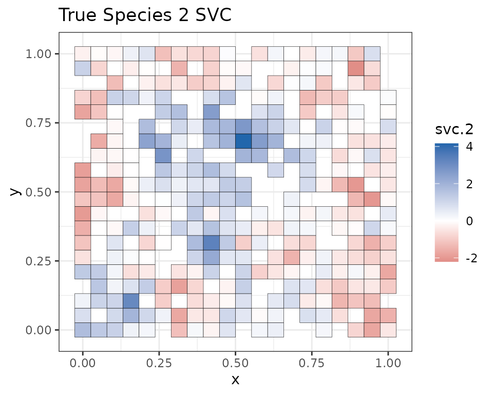
ggplot(plot.dat, aes(x = x, y = y, fill = svc.est.2)) +
  geom_tile(col = 'black') +
  scale_fill_gradient2(midpoint = 0, low = '#B2182B', mid = 'white',
                       high = '#2166AC', na.value = NA) +
  theme_bw() +
  labs(title = 'Estimate Species 2 SVC')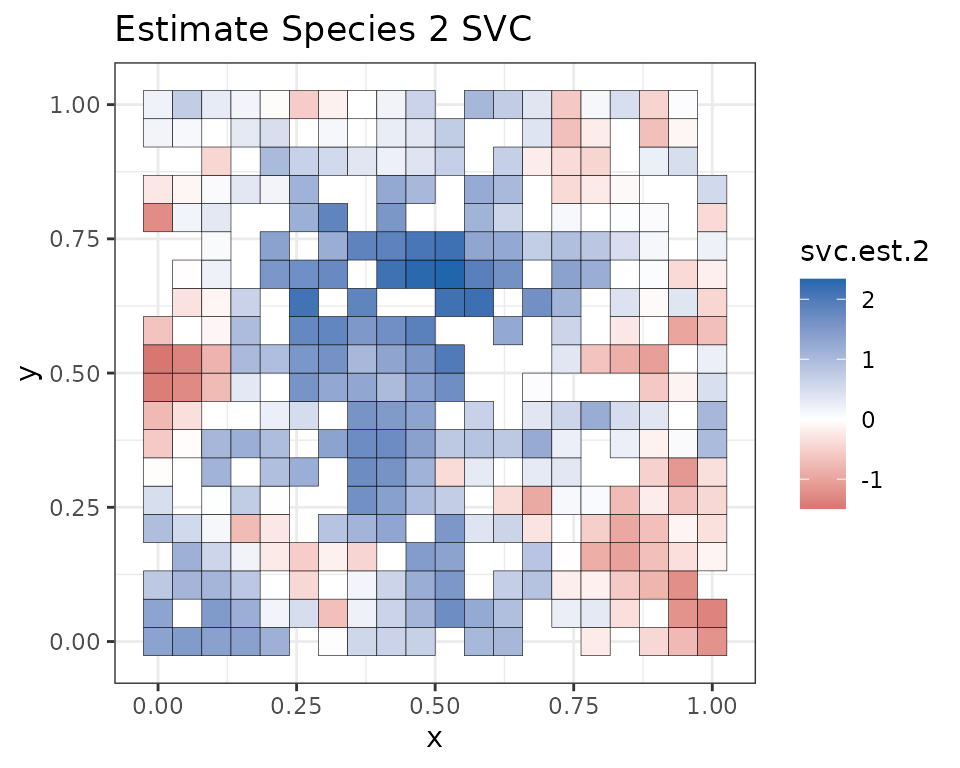
Posterior predictive checks
As before, we can use the ppcOcc() function to perform a
poseterior predictive check of the model as a goodness of fit
assessment.
# PPC with a chi-squared statistic, grouping the data by site
out.ms.ppc <- ppcOcc(out.ms, fit.stat = 'chi-squared', group = 1)
Currently on species 1 out of 6Currently on species 2 out of 6Currently on species 3 out of 6Currently on species 4 out of 6Currently on species 5 out of 6Currently on species 6 out of 6
summary(out.ms.ppc)
Call:
ppcOcc(object = out.ms, fit.stat = "chi-squared", group = 1)

Samples per Chain: 20000
Burn-in: 10000
Thinning Rate: 10
Number of Chains: 3
Total Posterior Samples: 3000

----------------------------------------
    Community Level
----------------------------------------
Bayesian p-value:  0.6878

----------------------------------------
    Species Level
----------------------------------------
sp1 Bayesian p-value: 0.738
sp2 Bayesian p-value: 0.663
sp3 Bayesian p-value: 0.6087
sp4 Bayesian p-value: 0.822
sp5 Bayesian p-value: 0.7237
sp6 Bayesian p-value: 0.5717
Fit statistic:  chi-squared
Model selection using WAIC
The waicOcc() function again allows us to calculate WAIC
to compare model performance across different models. As of v0.7.0,
waicOcc() also contains the by.sp argument for
all multi-species models, which if set to TRUE, will result
in a separate WAIC value returned for each species. This can be useful
for comparing performances of multi-species models for individual
species of interest. Note that the overall WAIC value is simply the sum
of all the individual species values.
# Overall WAIC
waicOcc(out.ms)
elpd pD WAIC
-2533.5939 208.3908 5483.9693
# WAIC by species
waicOcc(out.ms, by.sp = TRUE)
elpd pD WAIC
1 -397.1727 15.26636 824.8781
2 -500.0378 38.07061 1076.2168
3 -479.0836 44.20221 1046.5716
4 -425.7760 38.92541 929.4027
5 -357.8041 55.93871 827.4856
6 -373.7197 15.98749 779.4144Prediction
Prediction is identical to the single-species SVC model. Below we predict at the 100 hold out locations and then compare the estimated means to the true values used to simulate the data.
# Predict occupancy at the 100 new sites
out.ms.pred <- predict(out.ms, X.pred, coords.pred)
----------------------------------------
Prediction description
----------------------------------------
Spatial Factor NNGP Multispecies Occupancy model with Polya-Gamma latent
variable fit with 300 observations.
Number of covariates 2 (including intercept if specified).
Number of spatially-varying covariates 2 (including intercept if specified).
Using the exponential spatial correlation model.
Using 5 nearest neighbors.
Using 2 latent spatial factors.
Number of MCMC samples 3000.
Predicting at 100 non-sampled locations.
Source compiled with OpenMP support and model fit using 1 threads.
-------------------------------------------------
Predicting
-------------------------------------------------
Location: 100 of 100, 100.00%
Generating latent occupancy state
str(out.ms.pred)List of 6
$ z.0.samples : num [1:3000, 1:6, 1:100] 1 1 1 1 1 1 1 1 1 1 ...
$ w.0.samples : num [1:3000, 1:2, 1:100, 1:2] 0.1323 1.0731 -0.0471 -0.8771 -0.2433 ...
$ psi.0.samples: num [1:3000, 1:6, 1:100] 0.937 0.97 0.973 0.647 0.767 ...
$ run.time : 'proc_time' Named num [1:5] 1.5 1.64 1.6 0 0
..- attr(*, "names")= chr [1:5] "user.self" "sys.self" "elapsed" "user.child" ...
$ call : language predict.svcMsPGOcc(object = out.ms, X.0 = X.pred, coords.0 = coords.pred)
$ object.class : chr "svcMsPGOcc"
- attr(*, "class")= chr "predict.svcMsPGOcc"
# Use the getSVCSamples() function to extract the SVC values
# at the prediction locations
svc.pred.samples <- getSVCSamples(out.ms, pred.object = out.ms.pred)
# Get median and 95% CIs of the SVC for the covariate for each species
svc.pred.quants <- apply(svc.pred.samples[["occ.cov.1"]], c(2, 3), quantile,
                         probs = c(0.025, 0.5, 0.975))
# Plot results for one species
plot(svc.true.pred[2, ], svc.pred.quants[2, 2, ], pch = 19,
     ylim = c(min(svc.pred.quants[1, 2, ]), max(svc.pred.quants[3, 2, ])),
     xlab = "True", ylab = "Fit", main = 'Spatially-varying svc')
abline(0, 1)
arrows(svc.true.pred[2, ], svc.pred.quants[2, 2, ], svc.true.pred[2, ], col = 'gray',
       svc.pred.quants[1, 2, ], length = 0.02, angle = 90)
arrows(svc.true.pred[2, ], svc.pred.quants[1, 2, ], svc.true.pred[2, ], col = 'gray',
       svc.pred.quants[3, 2, ], length = 0.02, angle = 90)
points(svc.true.pred[2, ], svc.pred.quants[2, 2, ], pch = 19)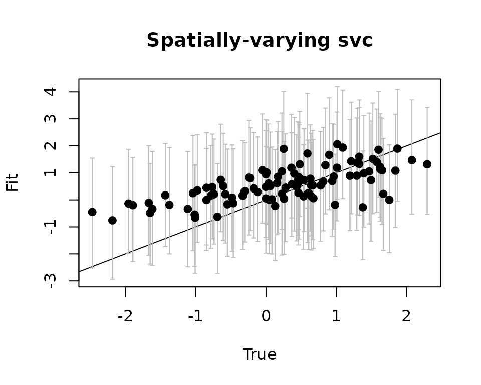
Multi-species multi-season spatially varying coefficient occupancy models
Example coming soon… See the help page for svcTMsPGOcc()
for a bare bones example for fitting multi-species, multi-season
spatially varying coefficient occupancy models.